Note
Go to the end to download the full example code.
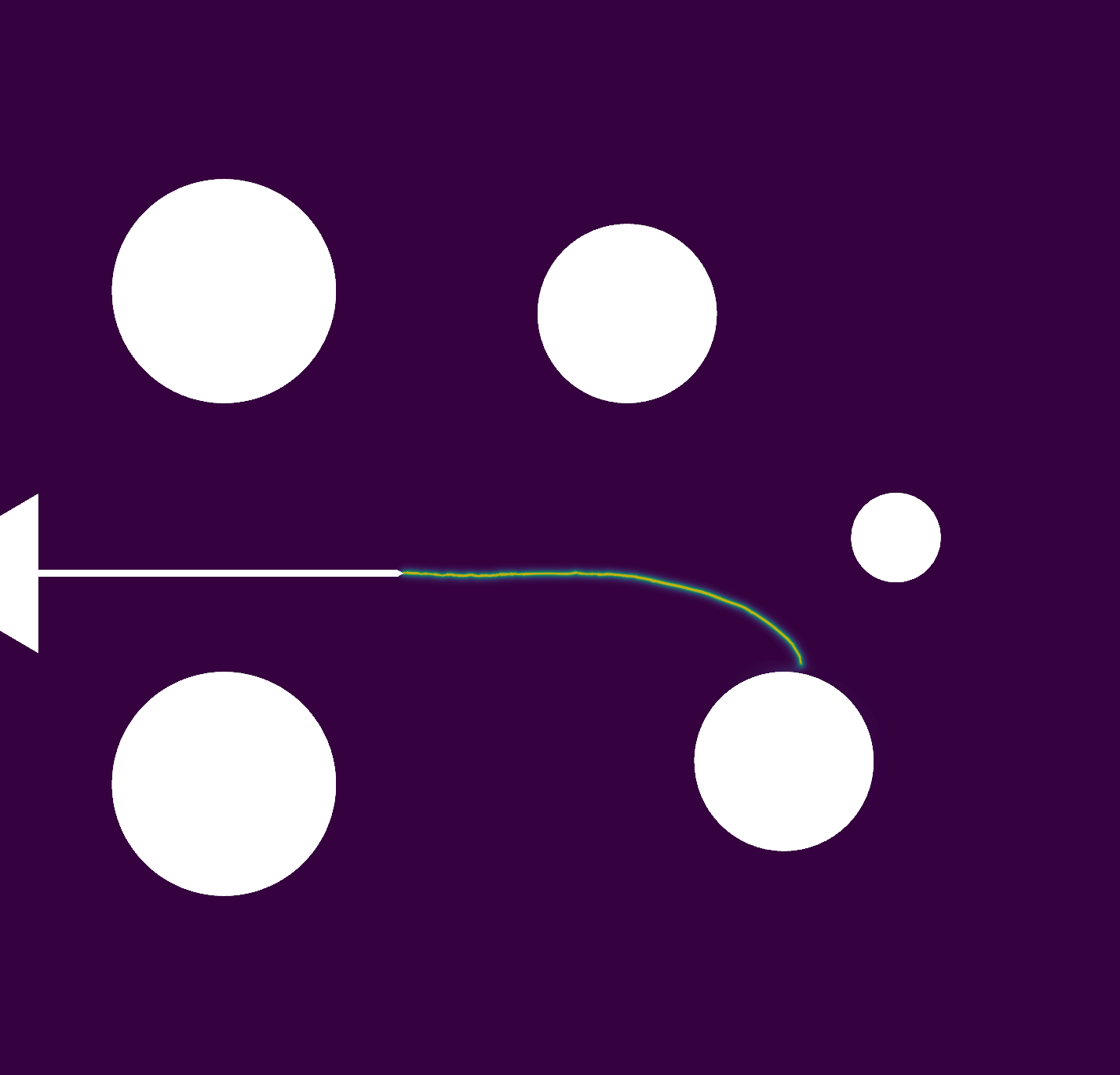
Length Scale Parameter Study for Phase-Field Fracture#
This script analyzes the influence of the length scale parameter on phase-field fracture simulations. The length scale parameter (\(l\)) is a critical regularization parameter in phase-field models that controls the width of the diffuse crack interface. It represents a balance between model accuracy and computational efficiency:
Physical significance: \(l\) approximates the fracture process zone width
Numerical role: Regularizes the sharp crack discontinuity into a diffuse damage field
Convergence properties: As \(l \rightarrow 0\), the phase-field model converges to the sharp crack solution
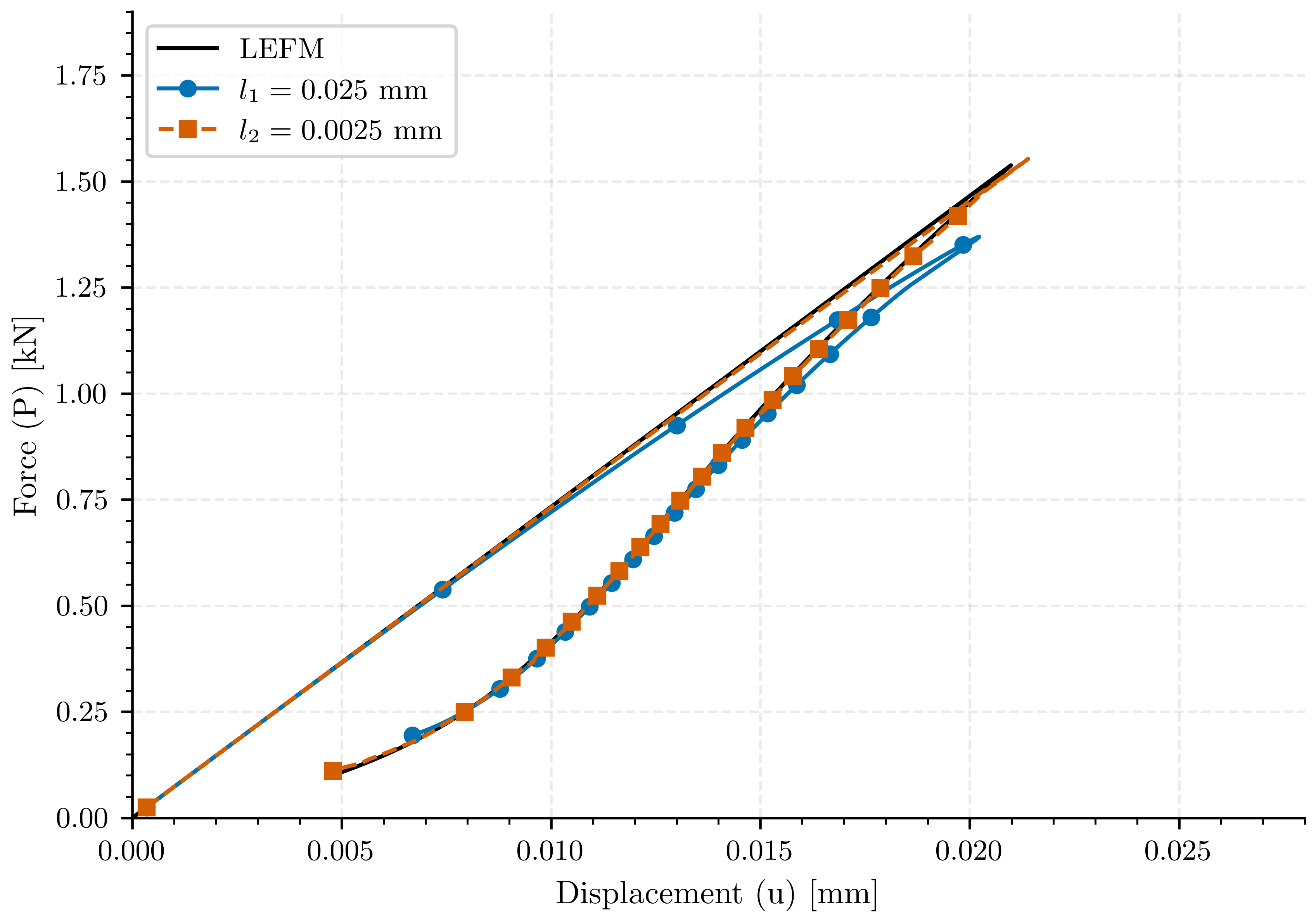
In this study, we compare two different length scale parameters for the central cracked tension specimen:
\(l_1 = 0.025\) mm: Coarser diffuse interface (computationally more efficient)
\(l_2 = 0.0025\) mm: Finer diffuse interface (more accurate, but computationally intensive)
For each length scale, we analyze three different initial crack lengths (\(a_0\)): 0.3 mm, 0.5 mm, and 0.7 mm, with the mesh size refined proportionally to the length scale parameter (\(h \approx 0.4l\)) to ensure adequate resolution of the diffuse interface.
The analysis focuses on several key relationships:
Crack surface evolution: How displacement relates to crack surface area (gamma)
Force-displacement response: Load-carrying capacity during crack propagation
Compliance-crack area: Comparison with Linear Elastic Fracture Mechanics (LEFM) predictions
Correction methods: Evaluating different approaches to correct the phase-field crack surface measurement
Through this comprehensive comparison, we demonstrate that properly calibrated phase-field models can accurately recover the LEFM solution, regardless of the length scale used, when appropriate correction factors are applied.
To examine the detailed setup and input files for each simulation, refer to the following links:
\(a_0\) |
\(l_1 = 0.025\) mm |
\(l_2 = 0.0025\) mm |
|---|---|---|
\(0.3\) mm |
||
\(0.5\) mm |
||
\(0.7\) mm |
Import necessary libraries#
import numpy as np
import pandas as pd
import matplotlib.pyplot as plt
import pyvista as pv
import os
import sys

sys.path.insert(0, os.path.abspath('../../'))
plt.style.use('../../graph.mplstyle')
import plot_config as pcfg

results_folder = "results_compare_lenght_scale"
if not os.path.exists(results_folder):
    os.makedirs(results_folder)
Load results#
Once the simulation finishes, the results are loaded from the results folder. The AllResults class takes the folder path as an argument and stores all the results, including logs, energy, convergence, and DOF files. Note that it is possible to load results from other results folders to compare results. It is also possible to define a custom label and color to automate plot labels.
simulation_1 = pd.read_csv("../Phase_Field_Central_Cracked/results_1_a03_l1/results.pff", delimiter="\t", comment="#", header=0)
simulation_1_bourdin = pd.read_csv("../Phase_Field_Central_Cracked/results_1_a03_l1/results_corrected_bourdin.pff", delimiter="\t", comment="#", header=0)
label_1 = r"$a=0.3$ mm, $l=l_1$"
label_1_a = r"$a_0=0.3$ mm"
label_1_l = r"$l_1=0.025$ mm"
color_1 = pcfg.color_blue
a01 = 0.3

simulation_2 = pd.read_csv("../Phase_Field_Central_Cracked/results_2_a03_l2/results.pff", delimiter="\t", comment="#", header=0)
simulation_2_bourdin = pd.read_csv("../Phase_Field_Central_Cracked/results_2_a03_l2/results_corrected_bourdin.pff", delimiter="\t", comment="#", header=0)
simulation_2_geometry = pd.read_csv("../Phase_Field_Central_Cracked/results_2_a03_l2/results_corrected_geometry.pff", delimiter="\t", comment="#", header=0)
label_2 = r"$a_0=0.3$ mm, $l=l_2$"
label_2_a = r"$a_0=0.3$ mm"
label_2_l = r"$l_2=0.0025$ mm"
color_2 = pcfg.color_orangered
a02 = 0.3

simulation_3 = pd.read_csv("../Phase_Field_Central_Cracked/results_3_a05_l1/results.pff", delimiter="\t", comment="#", header=0)
simulation_3_bourdin = pd.read_csv("../Phase_Field_Central_Cracked/results_3_a05_l1/results_corrected_bourdin.pff", delimiter="\t", comment="#", header=0)
label_3 = r"$a_0=0.5$ mm, $l=l_1$"
label_3_a = r"$a_0=0.5$ mm"
label_3_l = r"$l_1=0.025$ mm"
color_3 = pcfg.color_gold
a03 = 0.5

simulation_4 = pd.read_csv("../Phase_Field_Central_Cracked/results_4_a05_l2/results.pff", delimiter="\t", comment="#", header=0)
label_4 = r"$a_0=0.5$ mm, $l=l_2$"
label_4_a = r"$a_0=0.5$ mm"
label_4_l = r"$l_2=0.0025$ mm"
color_4 = pcfg.color_green
a04 = 0.5

simulation_5 = pd.read_csv("../Phase_Field_Central_Cracked/results_5_a07_l1/results.pff", delimiter="\t", comment="#", header=0)
simulation_5_bourdin = pd.read_csv("../Phase_Field_Central_Cracked/results_5_a07_l1/results_corrected_bourdin.pff", delimiter="\t", comment="#", header=0)
label_5 = r"$a_0=0.7$ mm, $l=l_1$"
label_5_a = r"$a_0=0.7$ mm"
label_5_l = r"$l_1=0.025$ mm"
color_5 = pcfg.color_purple
a05 = 0.7

simulation_6 = pd.read_csv("../Phase_Field_Central_Cracked/results_6_a07_l2/results.pff", delimiter="\t", comment="#", header=0)
label_6 = r"$a_0=0.7$ mm, $l=l_2$"
label_6_a = r"$a_0=0.7$ mm"
label_6_l = r"$l_2=0.0025$ mm"
color_6 = pcfg.color_brown
a06 = 0.7
From Linear elastic fracture mechanics theory LEFM: Center-Cracked Specimen
SCHEME_3 = np.loadtxt("../LEFM/results_central_cracked/center_cracked.lefm", delimiter="\t", skiprows=1)
a_lefm = SCHEME_3[:,0]
k_lefm = 1/SCHEME_3[:,2]
c_lefm = SCHEME_3[:,2]
dcda_lefm = SCHEME_3[:,3]
color_lefm = pcfg.color_black

results_lefm =  pd.read_csv("../LEFM/results_central_cracked/a0_03.lefm_problem", delimiter="\t", comment="#", header=0)

LABEL_LEFM = r"LEFM"
color_var = pcfg.color_black

# Calculate marker spacing for each dataset
markevery_1 = max(1, len(simulation_1["displacement"])//20)
markevery_2 = max(1, len(simulation_2["displacement"])//20)
markevery_3 = max(1, len(simulation_3["displacement"])//20)
markevery_4 = max(1, len(simulation_4["displacement"])//20)
markevery_5 = max(1, len(simulation_5["displacement"])//20)
markevery_6 = max(1, len(simulation_6["displacement"])//20)
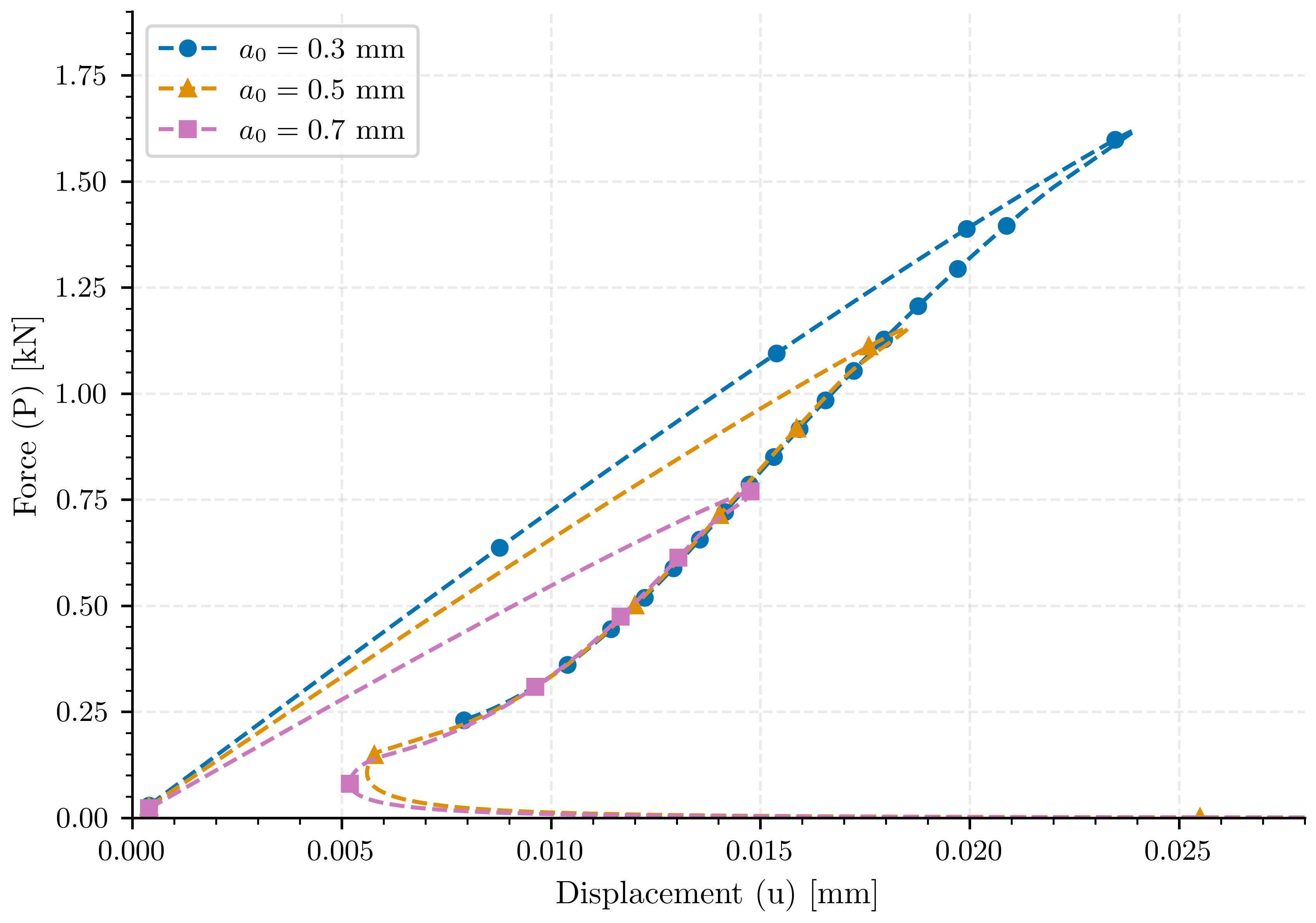
Plot: Displacement vs Force (Gamma)#
This plot shows the evolution of the crack surface area (gamma) as a function of the applied displacement. The crack surface area increases as the crack propagates. Note how the length scale parameter affects the curve’s shape: the smaller length scale (l2) produces a sharper transition at crack initiation, while the larger length scale (l1) shows a more gradual increase in damage.
fig, ax_l1_uf = plt.subplots()

ax_l1_uf.plot(simulation_1["displacement"], simulation_1["force"], color=color_1, linestyle='--', label=label_1_a, markevery=markevery_1, marker='o')
ax_l1_uf.plot(simulation_3["displacement"], simulation_3["force"], color=color_3, linestyle='--', label=label_3_a, markevery=markevery_3, marker='^')
ax_l1_uf.plot(simulation_5["displacement"], simulation_5["force"], color=color_5, linestyle='--', label=label_5_a, markevery=markevery_5, marker='s')

ax_l1_uf.set_xlim(left=0.0, right=0.028)
ax_l1_uf.set_ylim(bottom=0.0, top=1.9)
ax_l1_uf.set_xlabel(pcfg.displacement_label)
ax_l1_uf.set_ylabel(pcfg.force_label)
ax_l1_uf.legend()

plt.savefig(os.path.join(results_folder, "compare_all_l1_u_vs_force"))
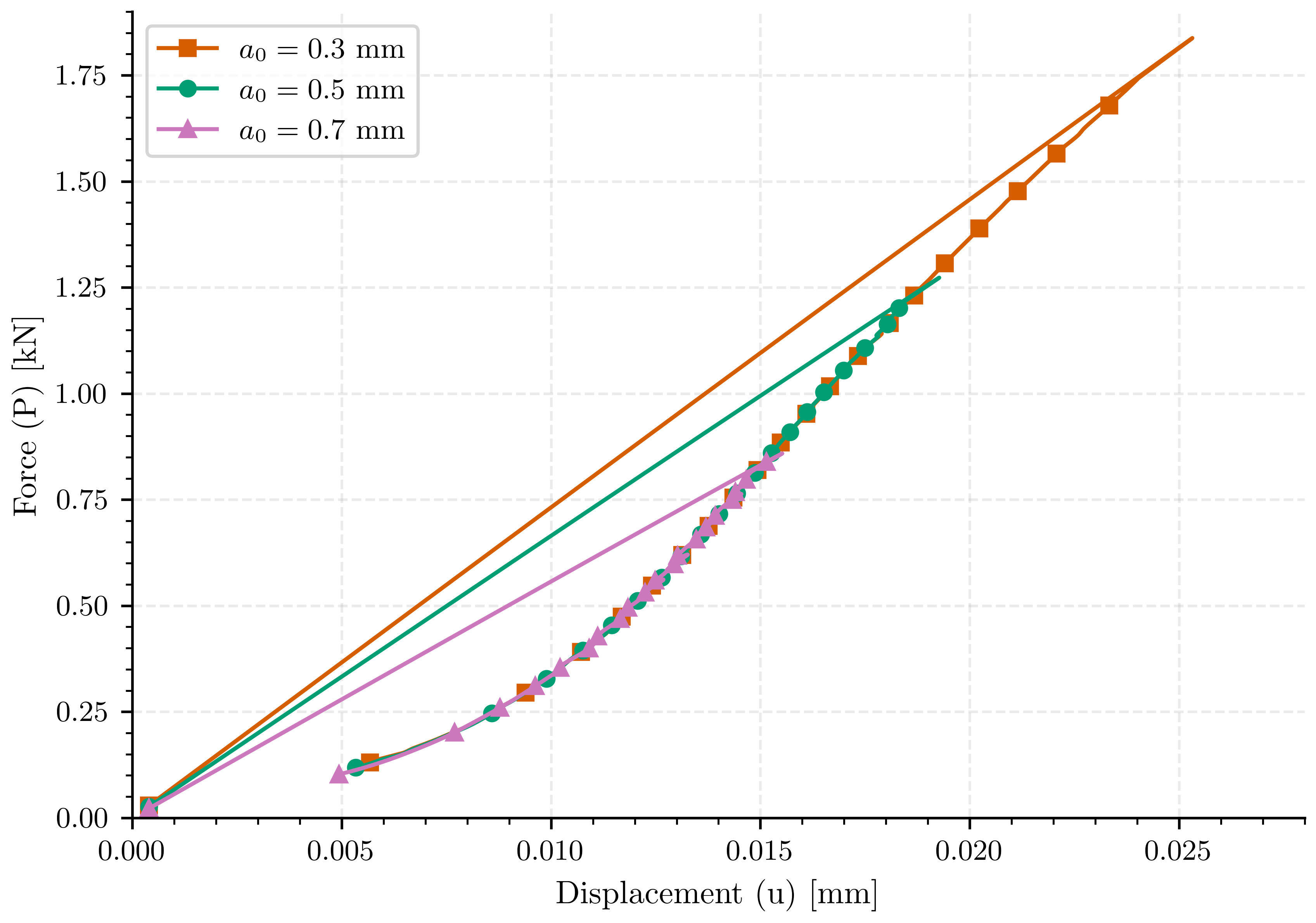
Plot: Displacement vs Force (Gamma)#
This plot shows the evolution of the crack surface area (gamma) as a function of the applied displacement. The crack surface area increases as the crack propagates. Note how the length scale parameter affects the curve’s shape: the smaller length scale (l2) produces a sharper transition at crack initiation, while the larger length scale (l1) shows a more gradual increase in damage.
fig, ax_l2_uf = plt.subplots()

ax_l2_uf.plot(simulation_2["displacement"], simulation_2["force"], color=color_2, linestyle='-', label=label_2_a, markevery=markevery_2, marker='s')
ax_l2_uf.plot(simulation_4["displacement"], simulation_4["force"], color=color_4, linestyle='-', label=label_4_a, markevery=markevery_4, marker='o')
ax_l2_uf.plot(simulation_6["displacement"], simulation_6["force"], color=color_5, linestyle='-', label=label_6_a, markevery=markevery_6, marker='^')

ax_l2_uf.set_xlim(left=0.0, right=0.028)
ax_l2_uf.set_ylim(bottom=0.0, top=1.9)
ax_l2_uf.set_xlabel(pcfg.displacement_label)
ax_l2_uf.set_ylabel(pcfg.force_label)
ax_l2_uf.legend()

plt.savefig(os.path.join(results_folder, "compare_all_l2_u_vs_force"))
Plot: Displacement vs Force#
fig, gamma = plt.subplots()
gamma.plot(results_lefm["u"], results_lefm["P"], color=color_lefm, linestyle='-', label=LABEL_LEFM)
gamma.plot(simulation_1_bourdin["displacement"], simulation_1_bourdin["force"], color=color_1, linestyle='-', label=label_1_l, markevery=markevery_1, marker='o')
gamma.plot(simulation_2_bourdin["displacement"], simulation_2_bourdin["force"], color=color_2, linestyle='--', label=label_2_l, markevery=markevery_2, marker='s')

gamma.set_xlim(left=0.0, right=0.028)
gamma.set_ylim(bottom=0.0, top=1.9)
gamma.set_xlabel(pcfg.displacement_label)
gamma.set_ylabel(pcfg.force_label)
gamma.legend(loc='upper left')
plt.savefig(os.path.join(results_folder, "compare_u_vs_force_l1_l2_lefm_corrected_gc"))
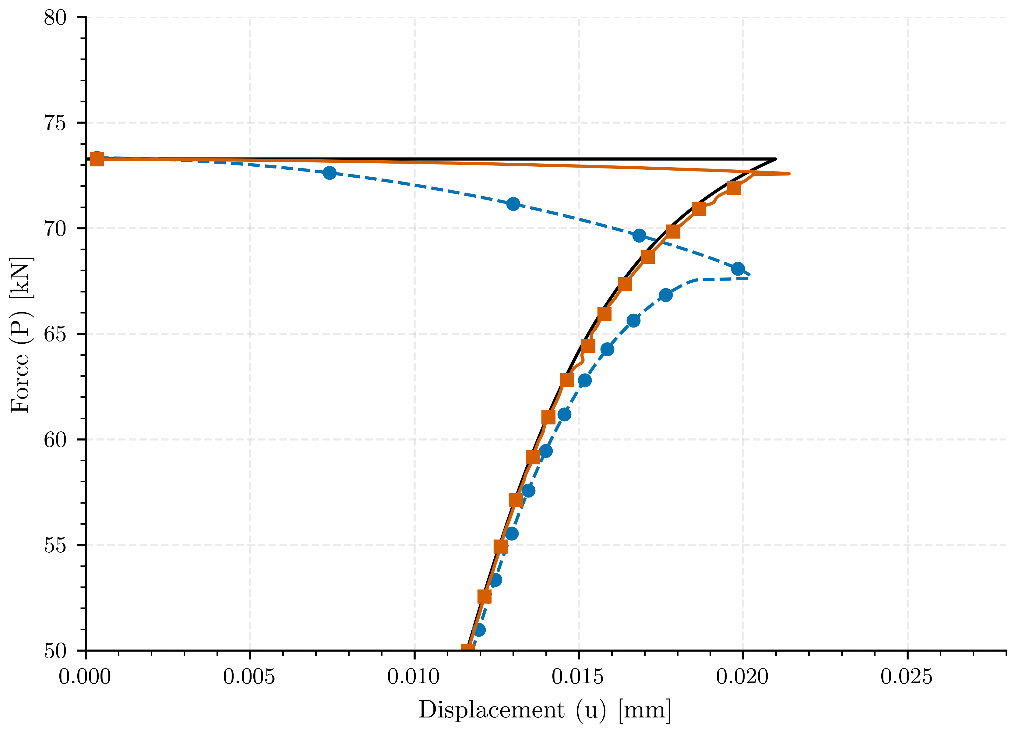
Plot: Displacement vs stiffness#
fig, gamma = plt.subplots()

gamma.plot(results_lefm["u"], results_lefm["P"]/results_lefm["u"], color=color_lefm, linestyle='-', label=LABEL_LEFM)
gamma.plot(simulation_1_bourdin["displacement"], 1/simulation_1_bourdin["compliance"], color=color_1, linestyle='--', label=label_1, markevery=markevery_1, marker='o')
gamma.plot(simulation_2_bourdin["displacement"], 1/simulation_2_bourdin["compliance"], color=color_2, linestyle='-', label=label_2, markevery=markevery_2, marker='s')

gamma.set_xlim(left=0.0, right=0.028)
gamma.set_ylim(bottom=50.0, top=80.0)
gamma.set_xlabel(pcfg.displacement_label)
gamma.set_ylabel(pcfg.force_label)
# gamma.legend()
plt.savefig(os.path.join(results_folder, "compare_displacement_vs_stiffness_l1_l2_lefm_corrected_gc"))
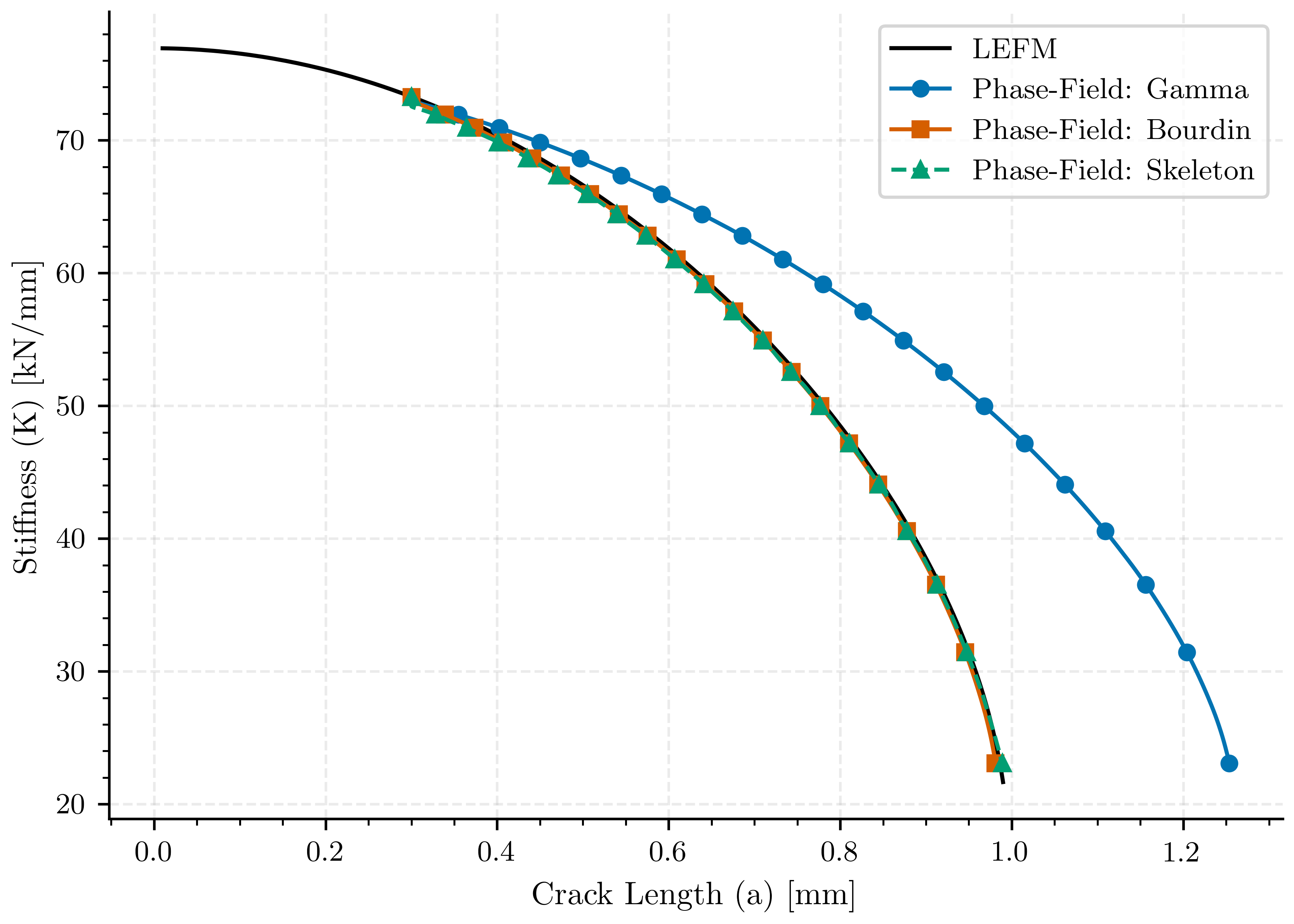
Plot: Gc-Corrected Crack Surface Area vs Stiffness#
This plot demonstrates the improved alignment between phase-field predictions and LEFM theory when applying the Gc-based crack surface correction method. The gamma_corrected_Gc value adjusts the raw crack surface area to account for the diffuse nature of the phase-field representation.
Key observations: 1. Corrected results align much better with the LEFM reference curve 2. Both length scales (l1 and l2) produce similar results after correction 3. This confirms that phase-field models can accurately predict structural
stiffness for varying crack lengths when properly calibrated
fig, ax_reaction = plt.subplots()

# LEFM reference
ax_reaction.plot(a_lefm, k_lefm, color=pcfg.color_black, linestyle='-', label=LABEL_LEFM)

ax_reaction.plot(simulation_2["gamma"], simulation_2["stiffness"], color=pcfg.color_blue, linestyle='-', label=r"Phase-Field: Gamma", markevery=markevery_2, marker='o')
ax_reaction.plot(simulation_2_bourdin["gamma"], simulation_2_bourdin["stiffness"], color=pcfg.color_orangered, linestyle='-', label=r"Phase-Field: Bourdin", markevery=markevery_2, marker='s')
ax_reaction.plot(simulation_2_geometry["gamma"], simulation_2_geometry["stiffness"], color=pcfg.color_green, linestyle='--', label=r"Phase-Field: Skeleton", markevery=markevery_2, marker='^')

ax_reaction.set_xlabel(pcfg.crack_length_label)
ax_reaction.set_ylabel(pcfg.stiffness_label)
ax_reaction.legend()

plt.savefig(os.path.join(results_folder, "gamma_compare_vs_k"))
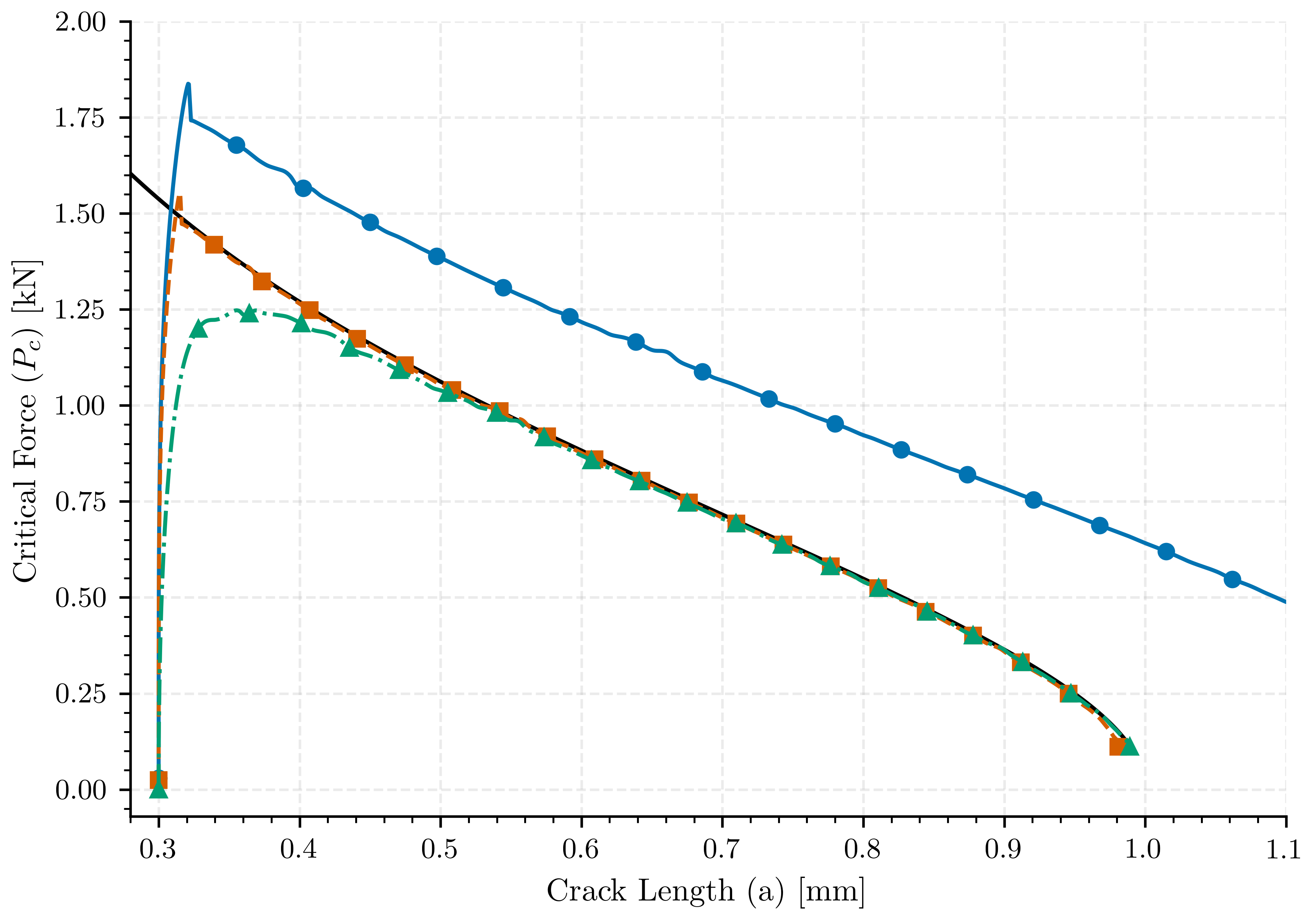
Crack length vs stiffness#
The stiffness as function of crack length is plotted for the three methods.
fig, ax0 = plt.subplots()

B=1
Gc=0.0027

factor_geo = (simulation_2["gamma"][0:len(simulation_2_geometry["gamma"])]-0.3)/(simulation_2_geometry["gamma"]-0.3)
pc_lefm = np.sqrt(2*B*Gc/dcda_lefm)
ax0.plot(a_lefm, pc_lefm, color=pcfg.color_black, linestyle='-', label=LABEL_LEFM)
ax0.plot(simulation_2["gamma"], np.sqrt(2*2*B*Gc/simulation_2["dCda"]), color=pcfg.color_blue, linestyle='-', label=pcfg.gamma_ref_label, markevery=markevery_2, marker='o')
ax0.plot(simulation_2_bourdin["gamma"], np.sqrt(2*2*B*Gc/simulation_2_bourdin["dCda"]), color=pcfg.color_orangered, linestyle='--', label=pcfg.gamma_bourdin_label, markevery=markevery_2, marker='s')
ax0.plot(simulation_2_geometry["gamma"], np.sqrt(2*2*B*Gc/simulation_2_geometry["dCda"]), color=pcfg.color_green, linestyle='-.', label=pcfg.gamma_geometry_label, markevery=markevery_2, marker='^')


ax0.set_xlim(left=0.28, right=1.1)
ax0.set_ylim(bottom=-0.07, top=2.0)
# Enhance plot aesthetics
ax0.set_xlabel(pcfg.crack_length_label)
ax0.set_ylabel(pcfg.critical_force_label)
# ax0.legend()

# Save the figure
plt.savefig(os.path.join(results_folder, "critical_force_vs_crack_length_pff"))

plt.show()
/home/docs/checkouts/readthedocs.org/user_builds/phasefieldfatigue/conda/stable/lib/python3.10/site-packages/pandas/core/arraylike.py:399: RuntimeWarning: invalid value encountered in sqrt
  result = getattr(ufunc, method)(*inputs, **kwargs)
Total running time of the script: (0 minutes 7.318 seconds)