
Note
Go to the end to download the full example code.
Three-Point Bending Specimen: Fracture and Fatigue Analysis#
This script performs a detailed fracture and fatigue analysis of an ASTM E-399-72 compact tension (CT) specimen using principles of Linear Elastic Fracture Mechanics (LEFM). It serves as a comprehensive educational and research tool, demonstrating the theoretical and numerical workflow from fundamental equations to result visualization.
Analysis Workflow:
Parameter Definition: Establishes material properties (e.g., Young’s modulus, fracture toughness) and specimen geometry based on the ASTM standard.
Geometric Factor Calculation: Implements the standard polynomial function for the dimensionless geometry factor, \(f(a/W)\).
Compliance Calculation: Numerically computes the specimen’s compliance, \(C(a)\), by integrating the energy release rate, which is derived from the geometry factor. This step is crucial for linking stress-based and energy-based fracture criteria.
Fatigue Life Analysis: * Calculates the stress intensity factor range, \(\Delta K\), using two
equivalent LEFM methods: a. Direct Method: Using the standard geometry factor, \(f(a/W)\). b. Compliance Method: Using the derivative of compliance, \(dC/da\).
Compares the results of both methods to verify the theoretical consistency.
Integrates Paris’ Law, \(da/dN = C_{\text{Paris}}(\Delta K)^n\), to predict the fatigue life, plotting the crack length as a function of the number of cycles.
Verification and Visualization: Generates plots to compare the different calculation methods and validates them against external experimental data.
Theoretical Background:
The analysis is based on the following key LEFM equations, which are also detailed in the accompanying scientific paper:
Stress Intensity Factor (SIF):
\[K_I = \frac{P}{B\sqrt{W}} f\left(\frac{a}{W}\right)\]Energy Release Rate and Compliance:
\[G = \frac{P^2}{2B} \frac{dC}{da} = \frac{K_I^2}{E'}\]Fatigue Crack Growth (Paris’ Law):
\[\frac{da}{dN} = C_{\text{Paris}} (\Delta K)^n\]
This script demonstrates how these foundational concepts are applied to a standard test case, providing a bridge between theory and practical implementation.
Import necessary libraries#
import numpy as np
import matplotlib.pyplot as plt
import matplotlib.image as mpimg
import os
import shutil
import sys

sys.path.insert(0, os.path.abspath('../../'))
plt.style.use('../../graph.mplstyle')
import plot_config as pcfg

img = mpimg.imread('images/three_point_bending.png')  # or .jpg, .tif, etc.
plt.imshow(img)
plt.axis('off')

results_folder = "results_three_point"
if os.path.exists(results_folder):
    shutil.rmtree(results_folder)
os.makedirs(results_folder, exist_ok=True)

# Colors reference from plot_config
color_main = pcfg.color_blue
color_secondary = pcfg.color_orangered
color_tertiary = pcfg.color_gold
color_quaternary = pcfg.color_green
color_analytical = pcfg.color_black
Parameters definition#
Define material and specimen parameters
E = 20.8 # Young's modulus (kN/mm^2)
nu = 0.3 # Poisson's ratio (-)
Gc = 0.0005 # Critical strain energy release rate (kN/mm)
m = 2.5 # Paris' Law exponent (-)
Cparis = 1.02*10**(-11) * 10**(3*m) # Paris' Law constant [mm^((2+3m)/2) / (cycle kN^m)]
Ep = E / (1.0 - nu**2) # Plane strain modulus (kN/mm^2)
# %
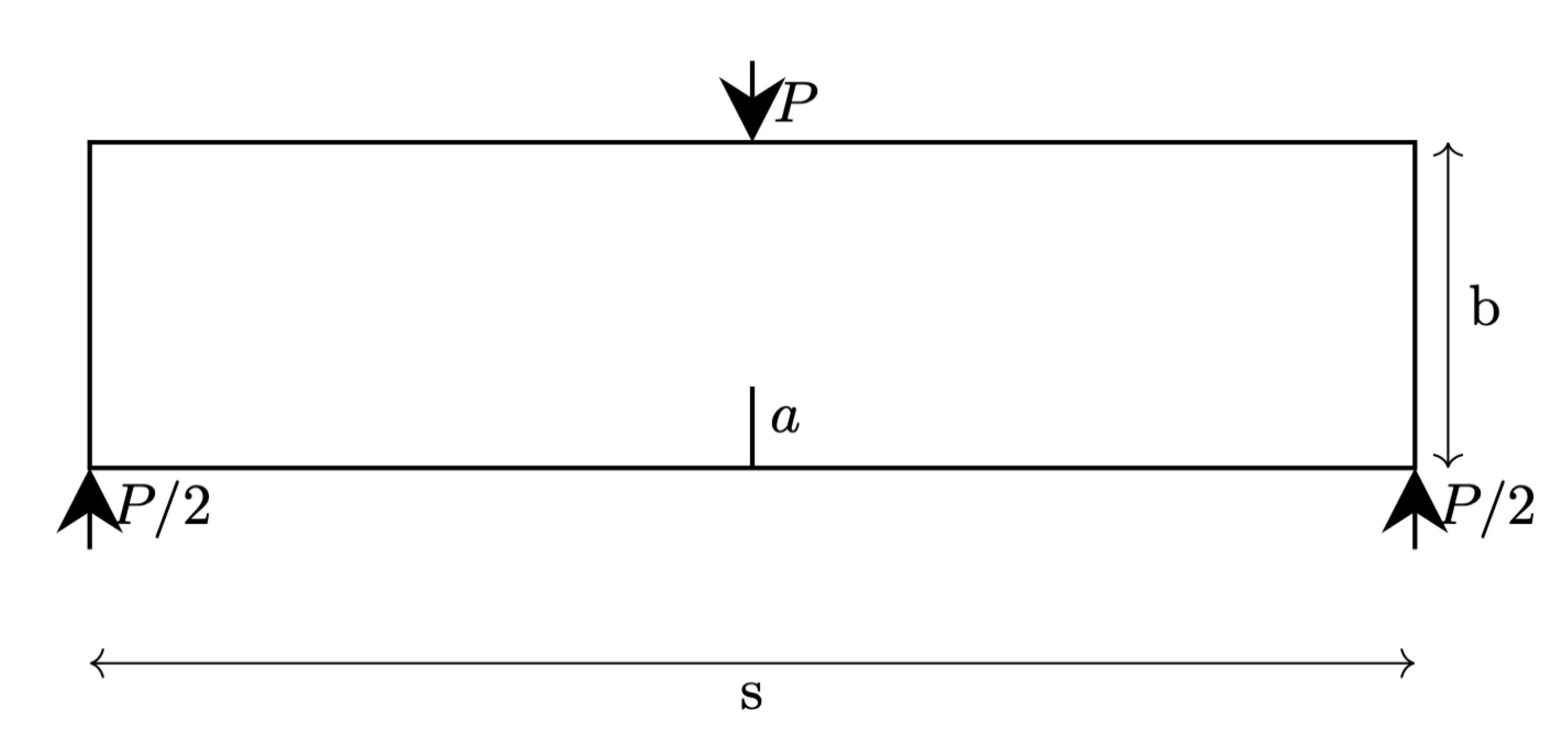
# Define specimen geometry
b = 1.0 # Characteristic width of the specimen (mm)
B = 1.0 # Thickness (mm)
s = 8.0
# %
# Crack length range and increment
a0 = 0.001 * b # Initial crack length (mm)
af = 0.95 * b # Final crack length (mm)
da = 0.0001 * b # Small increment for high-accuracy numerical integration (mm)
a = np.arange(a0, af, da) # Array of crack lengths (mm)
3. Geometric Factor and Compliance Calculation#
This section defines the geometry factor function and uses it to compute the specimen’s compliance via numerical integration.
def geometry_factor(a, b):
    """
    Calculates the dimensionless geometry factor f(a/b)
    """
    x = a / b
    s_div_b = 8.0
    numerator = np.sqrt(np.pi) * 3 * s_div_b * np.sqrt(x)
    denominator = 2.0
    polynomial = 1.106 - 1.552 * x + 7.71 * x**2 - 13.53 * x**3 + 14.23 * x**4
    return (numerator / denominator) * polynomial

# Calculate the geometric factor for the entire range of crack lengths
f_geometric = geometry_factor(a, b)
Calculate the critical force#
Critical force (\(P_c\)) based on LEFM
P_c = B * np.sqrt(b) * np.sqrt(Ep * Gc) / f_geometric
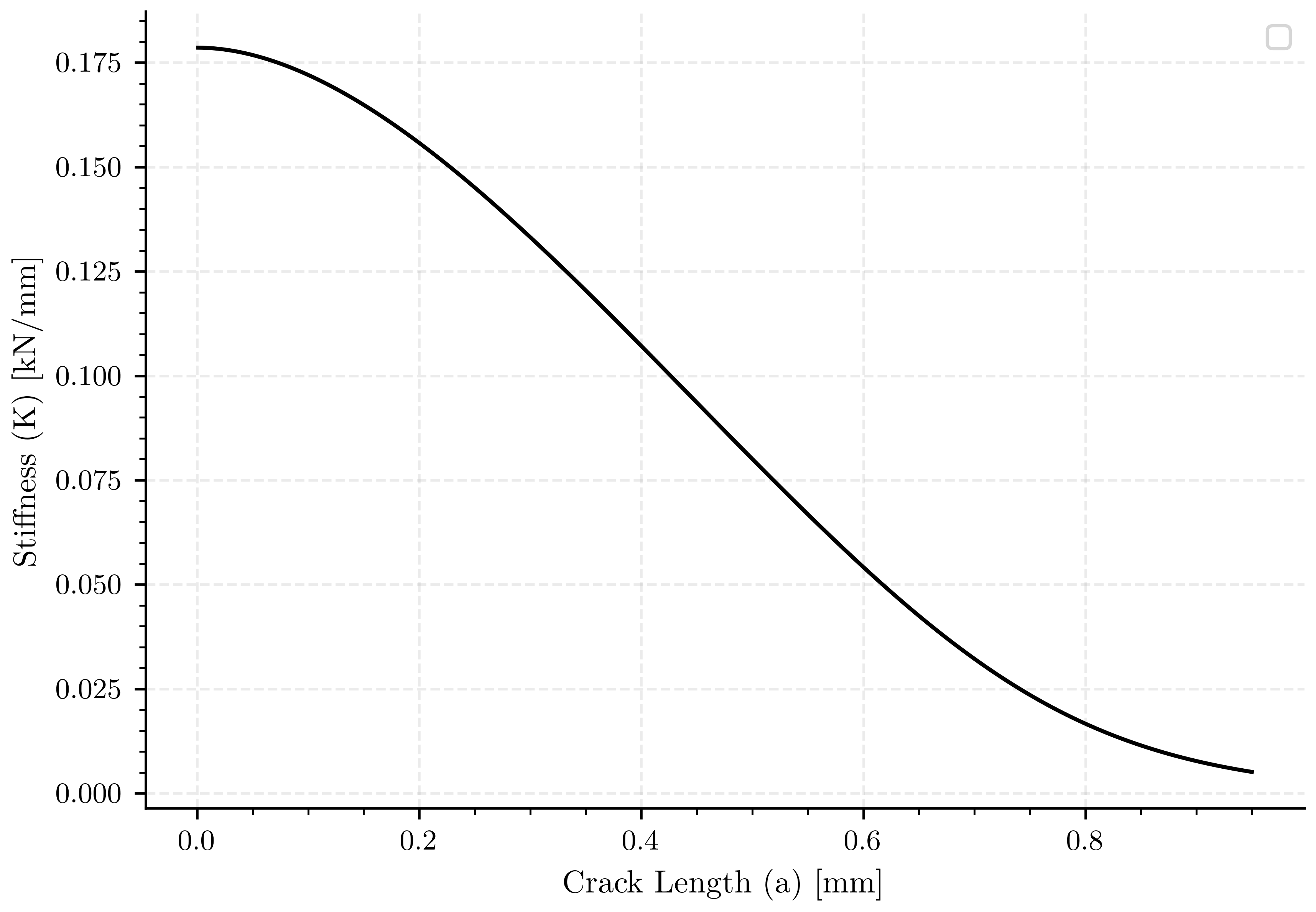
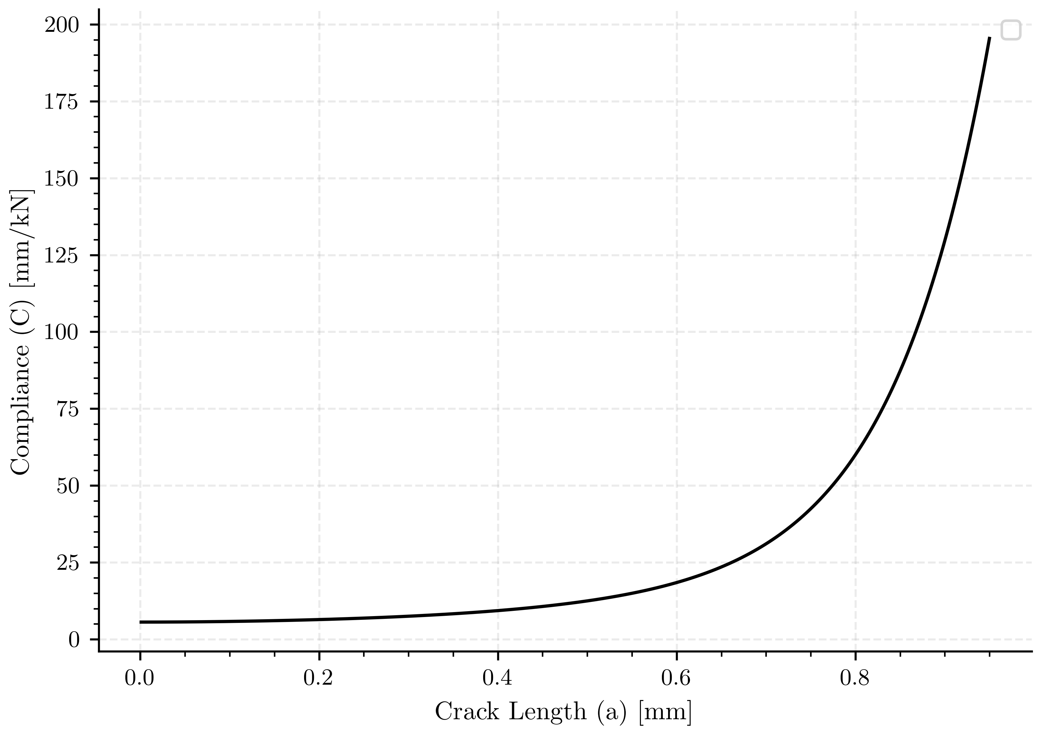
Compliance and stiffness calculations#
Compliance (C) and stiffness (K) are calculated using numerical integration The compliance of the specimen witout crack is given by:
I = B * b**3 / 12.0
C0 = s**3 / (48 * Ep * I)
K0 = 1.0 / C0
C0 = 1.0/K0

# Define integration function using trapezoidal or Simpson's rule
from scipy.integrate import cumulative_trapezoid, cumulative_simpson

# Calculate compliance (C) and stiffness (K)
C = C0/B * (1 + 2.0 / (C0 * Ep * b) * cumulative_trapezoid(f_geometric**2, a, initial=0))
K = 1.0 / C  # Stiffness is inverse of compliance
Plot: Stiffness (\(K\)) vs. crack length (\(a\))#
fig, ax1 = plt.subplots()

ax1.plot(a, K, color=color_analytical, linestyle='-')  # Plot K vs. a

ax1.set_xlabel(pcfg.crack_length_label)  # Label for crack length
ax1.set_ylabel(pcfg.stiffness_label)  # Label for stiffness
ax1.legend()
/home/docs/checkouts/readthedocs.org/user_builds/phasefieldfatigue/checkouts/stable/examples/LEFM/plot_three_point.py:170: UserWarning: No artists with labels found to put in legend.  Note that artists whose label start with an underscore are ignored when legend() is called with no argument.
  ax1.legend()

<matplotlib.legend.Legend object at 0x734c779697e0>
Plot: Compliance (\(C\)) vs. crack length (\(a\))#
fig, ax1 = plt.subplots()

ax1.plot(a, C, color=color_analytical, linestyle='-')  # Plot K vs. a

ax1.set_xlabel(pcfg.crack_length_label)  # Label for crack length
ax1.set_ylabel(pcfg.compliance_label)  # Label for compliance
ax1.legend()
/home/docs/checkouts/readthedocs.org/user_builds/phasefieldfatigue/checkouts/stable/examples/LEFM/plot_three_point.py:181: UserWarning: No artists with labels found to put in legend.  Note that artists whose label start with an underscore are ignored when legend() is called with no argument.
  ax1.legend()

<matplotlib.legend.Legend object at 0x734c633e1090>
dC/da term#
This term is calculated as the derivative of compliance with respect to crack length note that the crack prpagates symetrically yo the right and the left, so we use 2*a for the derivative.
dCda_numerical = np.gradient(C, B*a)

# %
# Also is possible to obtain the relation directly by the following formula
dCda = 2*Gc / P_c**2

# Simple test to verify that the numerical and analytical dC/da are close
try:
    # Use a relative tolerance of 5% because numerical differentiation can
    # have inaccuracies.
    np.testing.assert_allclose(dCda_numerical, dCda, rtol=1e-2)
    print("Validation successful: Numerical dC/da matches analytical dC/da"
          " within tolerance.")
except AssertionError as e:
    print("Validation failed: Numerical and analytical dC/da do not match."
          f"\n{e}")


fig, ax1 = plt.subplots()
ax1.plot(a, dCda, color=color_analytical, linestyle='-', label='Analytical')  # Plot analytical dC/da
ax1.plot(a, dCda_numerical, color=color_quaternary, linestyle='--', label='Numerical')  # Plot numerical dC/da

ax1.set_xlabel(pcfg.crack_length_label)  # Label for crack length
ax1.set_ylabel(pcfg.dCda_label)
ax1.legend()
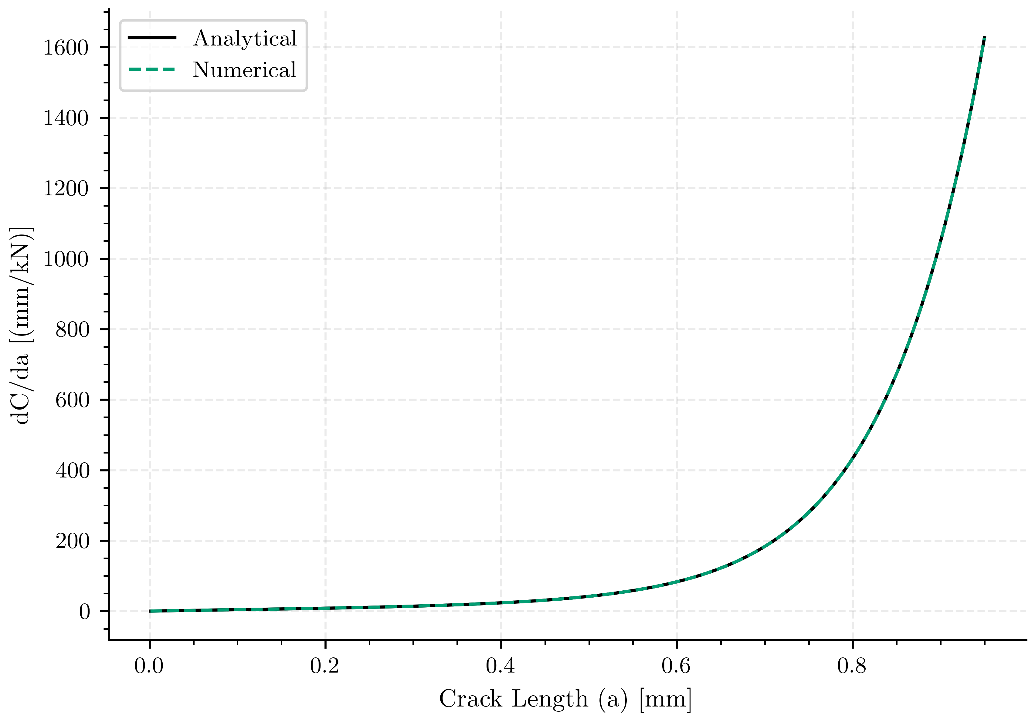
Validation failed: Numerical and analytical dC/da do not match.

Not equal to tolerance rtol=0.01, atol=0

Mismatched elements: 1 / 9490 (0.0105%)
Max absolute difference: 0.70998384
Max relative difference: 0.04984704
 x: array([5.069242e-02, 5.309865e-02, 5.790976e-02, ..., 1.623903e+03,
       1.625322e+03, 1.626032e+03])
 y: array([4.828553e-02, 5.309931e-02, 5.791043e-02, ..., 1.623903e+03,
       1.625322e+03, 1.626742e+03])

<matplotlib.legend.Legend object at 0x734c76e34370>
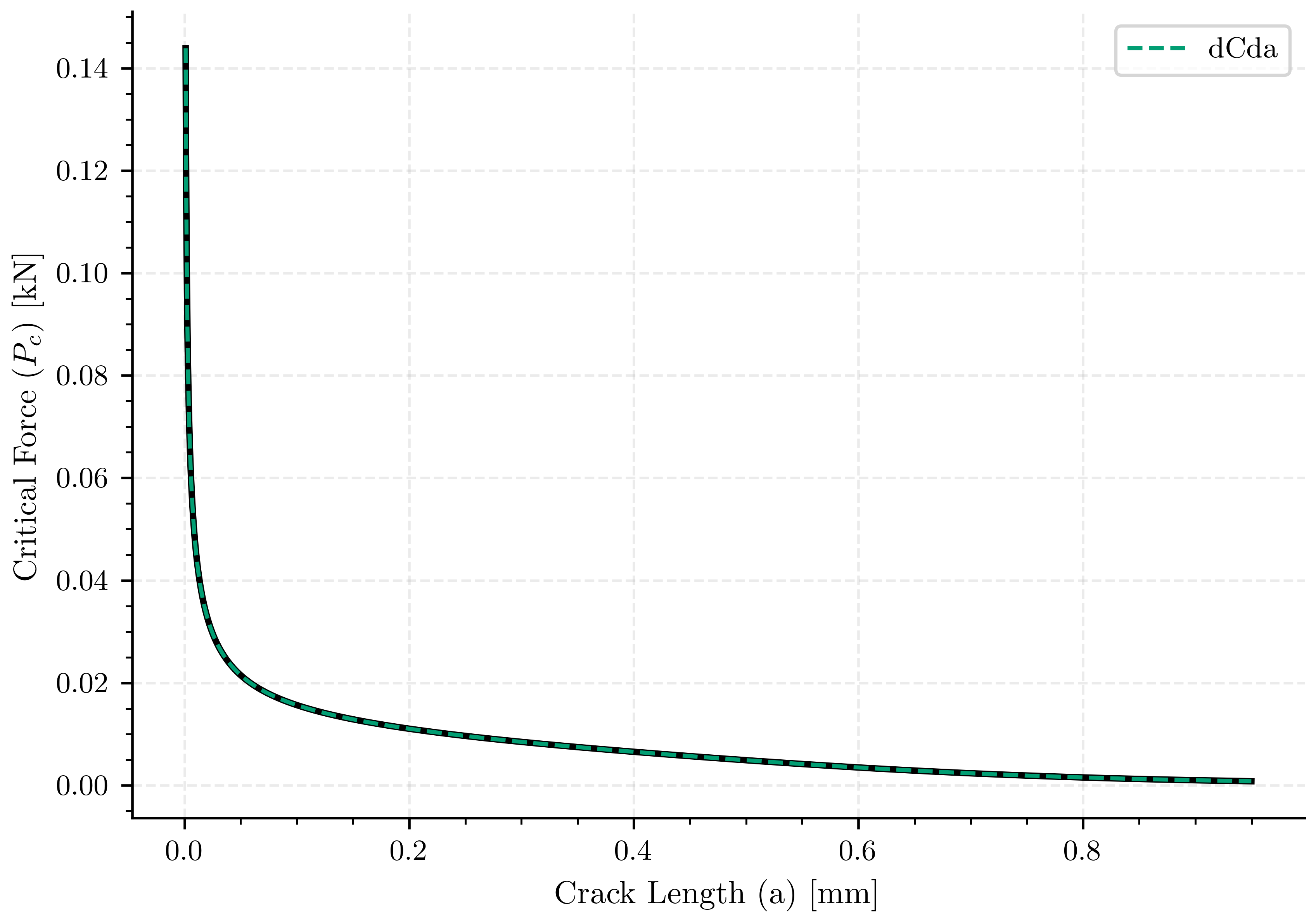
Plot: Critical force (\(P_c\)) vs. crack length (\(a\))#
fig, ax1 = plt.subplots()

ax1.plot(a, P_c, 'k-', color=color_analytical, linestyle='-', linewidth=2.0)  # Plot P_c vs. a
ax1.plot(a, np.sqrt(2.0 * Gc / dCda), 'y--',  color=color_quaternary, linestyle='--', label='dCda')
ax1.set_xlabel(pcfg.crack_length_label)  # Label for crack length
ax1.set_ylabel(pcfg.critical_force_label)  # Label for critical force
ax1.legend()
/home/docs/checkouts/readthedocs.org/user_builds/phasefieldfatigue/checkouts/stable/examples/LEFM/plot_three_point.py:219: UserWarning: linestyle is redundantly defined by the 'linestyle' keyword argument and the fmt string "k-" (-> linestyle='-'). The keyword argument will take precedence.
  ax1.plot(a, P_c, 'k-', color=color_analytical, linestyle='-', linewidth=2.0)  # Plot P_c vs. a
/home/docs/checkouts/readthedocs.org/user_builds/phasefieldfatigue/checkouts/stable/examples/LEFM/plot_three_point.py:219: UserWarning: color is redundantly defined by the 'color' keyword argument and the fmt string "k-" (-> color='k'). The keyword argument will take precedence.
  ax1.plot(a, P_c, 'k-', color=color_analytical, linestyle='-', linewidth=2.0)  # Plot P_c vs. a
/home/docs/checkouts/readthedocs.org/user_builds/phasefieldfatigue/checkouts/stable/examples/LEFM/plot_three_point.py:220: UserWarning: linestyle is redundantly defined by the 'linestyle' keyword argument and the fmt string "y--" (-> linestyle='--'). The keyword argument will take precedence.
  ax1.plot(a, np.sqrt(2.0 * Gc / dCda), 'y--',  color=color_quaternary, linestyle='--', label='dCda')
/home/docs/checkouts/readthedocs.org/user_builds/phasefieldfatigue/checkouts/stable/examples/LEFM/plot_three_point.py:220: UserWarning: color is redundantly defined by the 'color' keyword argument and the fmt string "y--" (-> color='y'). The keyword argument will take precedence.
  ax1.plot(a, np.sqrt(2.0 * Gc / dCda), 'y--',  color=color_quaternary, linestyle='--', label='dCda')

<matplotlib.legend.Legend object at 0x734c636bdba0>
Save results to file#
results = np.column_stack((a, K, P_c, dCda))
header = "a\tK\tPc\tdCda"
np.savetxt(os.path.join(results_folder, "results.lefm"),
           results, fmt="%.6e", delimiter="\t", header=header, comments="")
Specific curves#
def get_u_P(ap0, a, P_c, C):
    index_ap0 = np.argmin(np.abs(a - ap0))
    P_c_a0 = P_c[index_ap0]
    u_c_a0 = P_c_a0 * C[index_ap0]

    u = P_c[index_ap0:] * C[index_ap0:]
    P = P_c[index_ap0:]
    a = a[index_ap0:]

    u0 = np.linspace(0, u[0], 1000)
    u = np.concatenate((u0, u))
    P = np.concatenate((u0 / C[index_ap0], P))
    a = np.concatenate((u0 * 0 + a[0], a))
    W = Gc * (a - ap0)
    C = u / P
    E = P**2 * C / 2
    # E = P*u / 2
    return u, P, a, W, E, u_c_a0, P_c_a0

# %
# Define specific crack length points for the analysis
ap0_points = np.array([0.2*b, 0.5*b, 0.7*b])  # Specific crack length points
ap0_colors = np.array(["red", "blue", "green"])  # Colors for these points in plots
ap0_style = ["-", "--", "--"]  # Line styles for these points
ap0_label = np.array([f"$a_0$={ap0_points[0]} mm", f"$a_0$={ap0_points[1]} mm ", f"$a_0$={ap0_points[2]} mm"])  # Labels for legend
index_ap0 = np.zeros(len(ap0_points), dtype=int)  # Indices of these points in the crack length array

# Find the indices of the specific crack length points in the array
i = 0
for a_i in ap0_points:
    index_ap0[i] = np.argmin(np.abs(a - a_i))  # Find the closest index
    i += 1

u1, P1, a1, W1, E1, u_c_a01, P_c_a01 = get_u_P(ap0_points[0], a, P_c, C)
u2, P2, a2, W2, E2, u_c_a02, P_c_a02 = get_u_P(ap0_points[1], a, P_c, C)
u3, P3, a3, W3, E3, u_c_a03, P_c_a03 = get_u_P(ap0_points[2], a, P_c, C)


header_curves = "a\tu\tP\tstrain_energy\tfracture_energy"
results_1 = np.column_stack((a1, u1, P1, E1, W1))
np.savetxt(
    os.path.join(
        results_folder,
        f"a0_{str(ap0_points[0]).replace('.', '')}.lefm_problem"
    ),
    results_1, fmt="%.6e", delimiter="\t", header=header_curves, comments=""
)

results_2 = np.column_stack((a2, u2, P2, E2, W2))
np.savetxt(
    os.path.join(
        results_folder,
        f"a0_{str(ap0_points[1]).replace('.', '')}.lefm_problem"
    ),
    results_2, fmt="%.6e", delimiter="\t", header=header_curves, comments=""
)

results_3 = np.column_stack((a3, u3, P3, E3, W3))
np.savetxt(
    os.path.join(
        results_folder,
        f"a0_{str(ap0_points[2]).replace('.', '')}.lefm_problem"
    ),
    results_3, fmt="%.6e", delimiter="\t", header=header_curves, comments=""
)
/home/docs/checkouts/readthedocs.org/user_builds/phasefieldfatigue/checkouts/stable/examples/LEFM/plot_three_point.py:252: RuntimeWarning: invalid value encountered in divide
  C = u / P
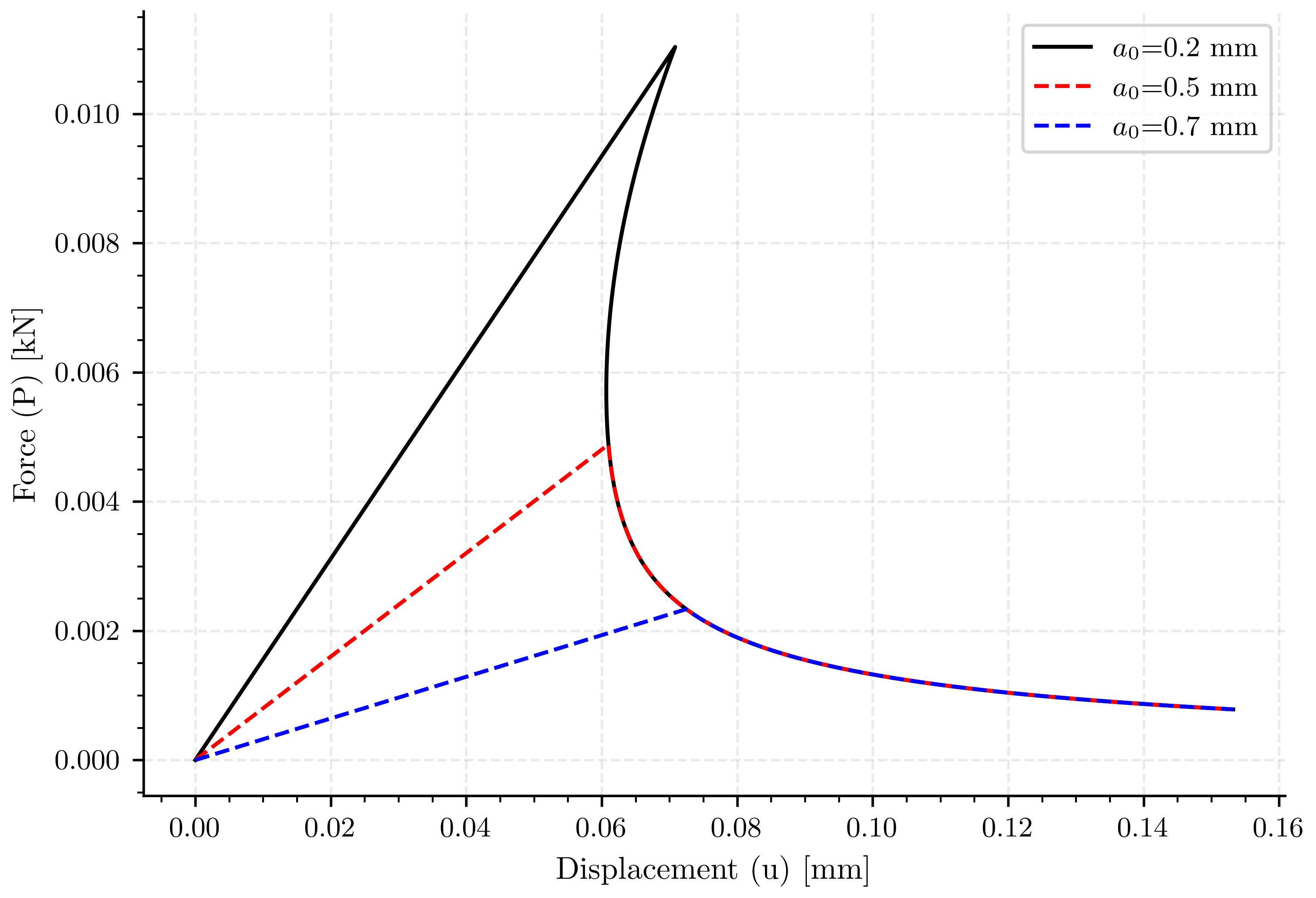
Plot: Displacement (\(u\)) vs. Force (\(P\))#
fig, ax1 = plt.subplots()

ax1.plot(u1, P1, 'k-', label=ap0_label[0])
ax1.plot(u2, P2, 'r--', label=ap0_label[1])
ax1.plot(u3, P3, 'b--', label=ap0_label[2])

ax1.set_xlabel(pcfg.displacement_label)
ax1.set_ylabel(pcfg.force_label)
ax1.legend()
<matplotlib.legend.Legend object at 0x734c63849bd0>
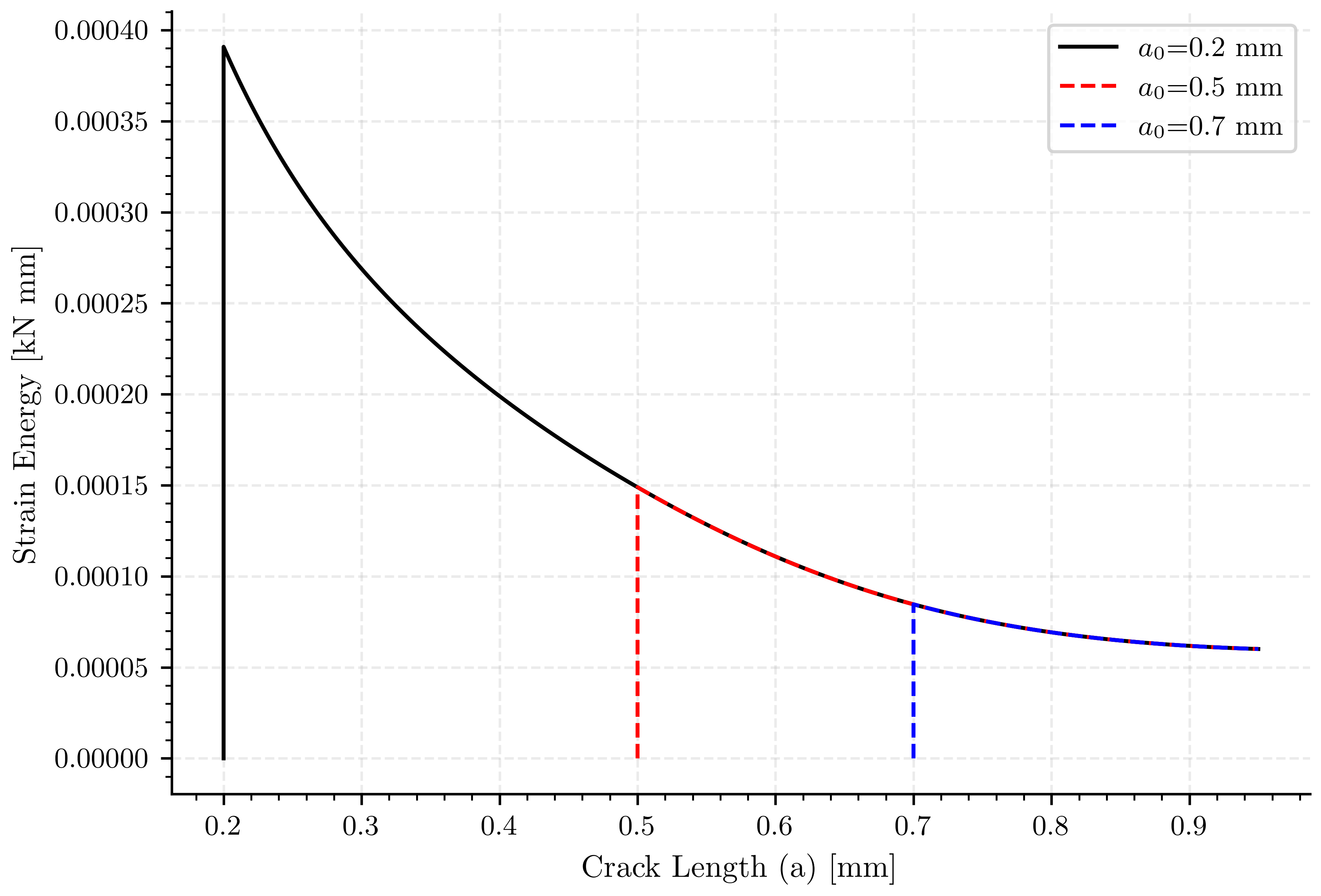
Plot: (\(a\)) vs. Energy (\(E\))#
fig, ax1 = plt.subplots()

ax1.plot(a1, E1, 'k-',  label=ap0_label[0])
ax1.plot(a2, E2, 'r--', label=ap0_label[1])
ax1.plot(a3, E3, 'b--', label=ap0_label[2])

ax1.set_xlabel(pcfg.crack_length_label)
ax1.set_ylabel(pcfg.strain_energy_label)
ax1.legend()
<matplotlib.legend.Legend object at 0x734c6355ef80>
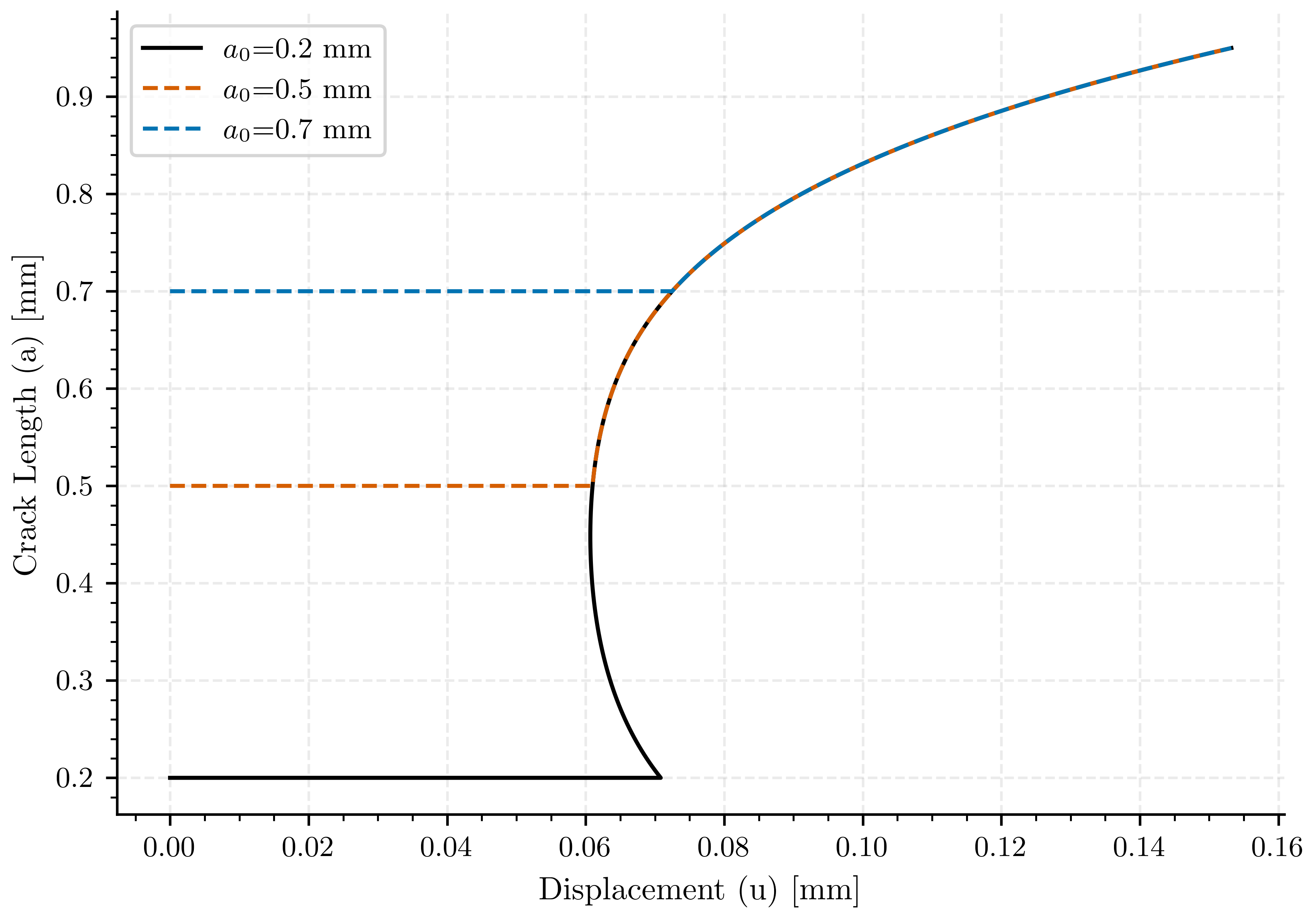
Energy calculations for a0=0.3 mm#
fig, ax1 = plt.subplots()

ax1.plot(u1, a1, color=color_analytical, linestyle='-', label=ap0_label[0])
ax1.plot(u2, a2, color=color_secondary, linestyle='--', label=ap0_label[1])
ax1.plot(u3, a3, color=color_main, linestyle='--', label=ap0_label[2])

ax1.set_xlabel(pcfg.displacement_label)
ax1.set_ylabel(pcfg.crack_length_label)
ax1.legend()
<matplotlib.legend.Legend object at 0x734c76e192d0>
Fatigue Life Calculation and Validation#
a0_fatigue = 0.2*b # Initial crack length [mm]
af_fatigue = 0.9*b # Final crack length [mm]
To perform the fatigue analysis in that range, will be needed to tlice the arrays to obtain the values of the compliance and crack area in that range.
def slice_array_by_values(a, value_1, value_2):
    """
    Returns a slice of the array `a` between the indices of the nearest values to `value_1` and `value_2`.

    Parameters:
    a (numpy.ndarray): The input array.
    value_1 (float): The first value to find in the array.
    value_2 (float): The second value to find in the array.

    Returns:
    numpy.ndarray: A new array sliced between the indices of the nearest values to `value_1` and `value_2`.
    """
    # Find the indices of the nearest values
    index_1 = (np.abs(a - value_1)).argmin()
    index_2 = (np.abs(a - value_2)).argmin()

    # Ensure index_1 is less than index_2
    if index_1 > index_2:
        index_1, index_2 = index_2, index_1

    # Return the sliced array
    return index_1, index_2 + 1
Slice the arrays to obtain the fatigue region
i_o_1, i_f_1 = slice_array_by_values(a, a0_fatigue, af_fatigue)
a_fatigue = a[i_o_1:i_f_1]  # Crack lengths in the fatigue range
f_geometric_fatigue = f_geometric[i_o_1:i_f_1]
dCda_fatigue = dCda[i_o_1:i_f_1]  # Compliance derivative in the fatigue range

# This section calculates the fatigue life (number of cycles vs. crack length)
# using two theoretically equivalent LEFM approaches:
#
# 1. Stress-Based Method: Using the geometric factor f(a/W) to find Delta_K.
# 2. Energy-Based Method: Using the compliance derivative dC/da.
#
# The results are then compared to validate the numerical implementation.

# --- Fatigue Material Properties ---
AP = 3.6   # Applied cyclic force range (Delta_P) [kN]
Ni = 0     # Initial number of cycles

# --- Method 1: Fatigue Life from Geometric Factor ---
# Calculate the stress intensity factor range (Delta_K)
AK = AP / (B * np.sqrt(b)) * f_geometric_fatigue  # Stress intensity factor range
# Integrate Paris' Law: Nf = integral(1 / (C * (Delta_K)^m)) da
# For numerical stability, constant terms are pulled out of the integral.
Nf_f_geometric = Ni + 1/(Cparis * (AP/(B*np.sqrt(b)))**m) * \
    cumulative_trapezoid(1/(f_geometric_fatigue**m), a_fatigue, initial=0)
# Nf_f_geometric = Ni + cumulative_trapezoid(1 / (Cparis * AK**m), a, initial=0)

# --- Method 2: Fatigue Life from Compliance Derivative (dC/da) ---
# This uses the energy-based formulation of Paris' Law.
Nf_dCda = Ni + 1 / (Cparis * (Ep / (2 * B))**(m / 2) * AP**m) * \
    cumulative_trapezoid(1 / (dCda_fatigue*(B))**(m / 2), a_fatigue, initial=0)

# --- Validation Test ---
# Verify that both methods produce nearly identical results. A small tolerance
# is required to account for numerical errors from integration and differentiation.
try:
    # Use a relative tolerance of 1% (rtol=1e-2).
    np.testing.assert_allclose(Nf_f_geometric, Nf_dCda, rtol=1e-2)
    print("Validation successful: Fatigue life calculations from geometric"
          " factor and dC/da are consistent.")
except AssertionError as e:
    print("Validation FAILED: The two fatigue life calculation methods do not"
          f" match.\n{e}")
Validation successful: Fatigue life calculations from geometric factor and dC/da are consistent.
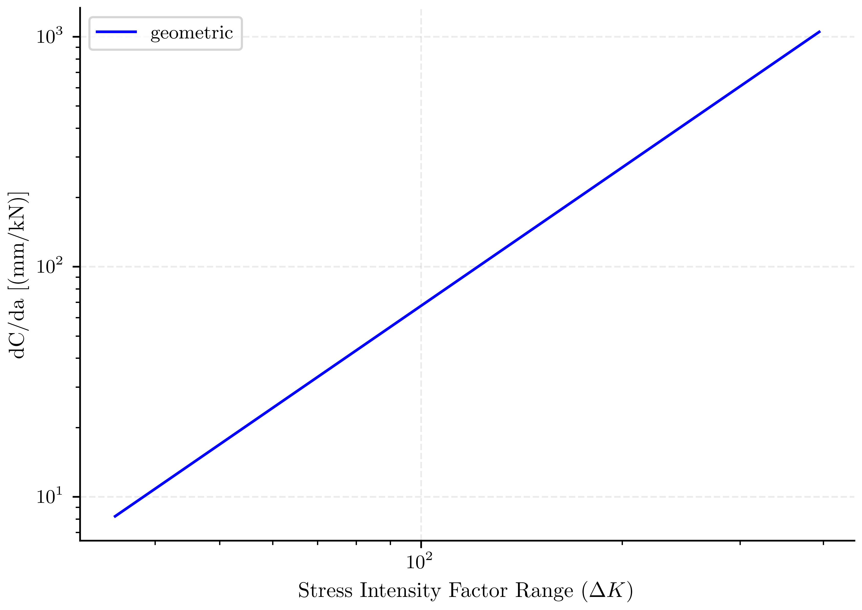
Plot: K Tada 2#
fig, ax1 = plt.subplots()

ax1.loglog(AK, dCda_fatigue, 'b-', label=r'geometric')

ax1.set_xlabel(pcfg.DeltaK_label)
ax1.set_ylabel(pcfg.dCda_label)
ax1.legend()
<matplotlib.legend.Legend object at 0x734c76b655a0>
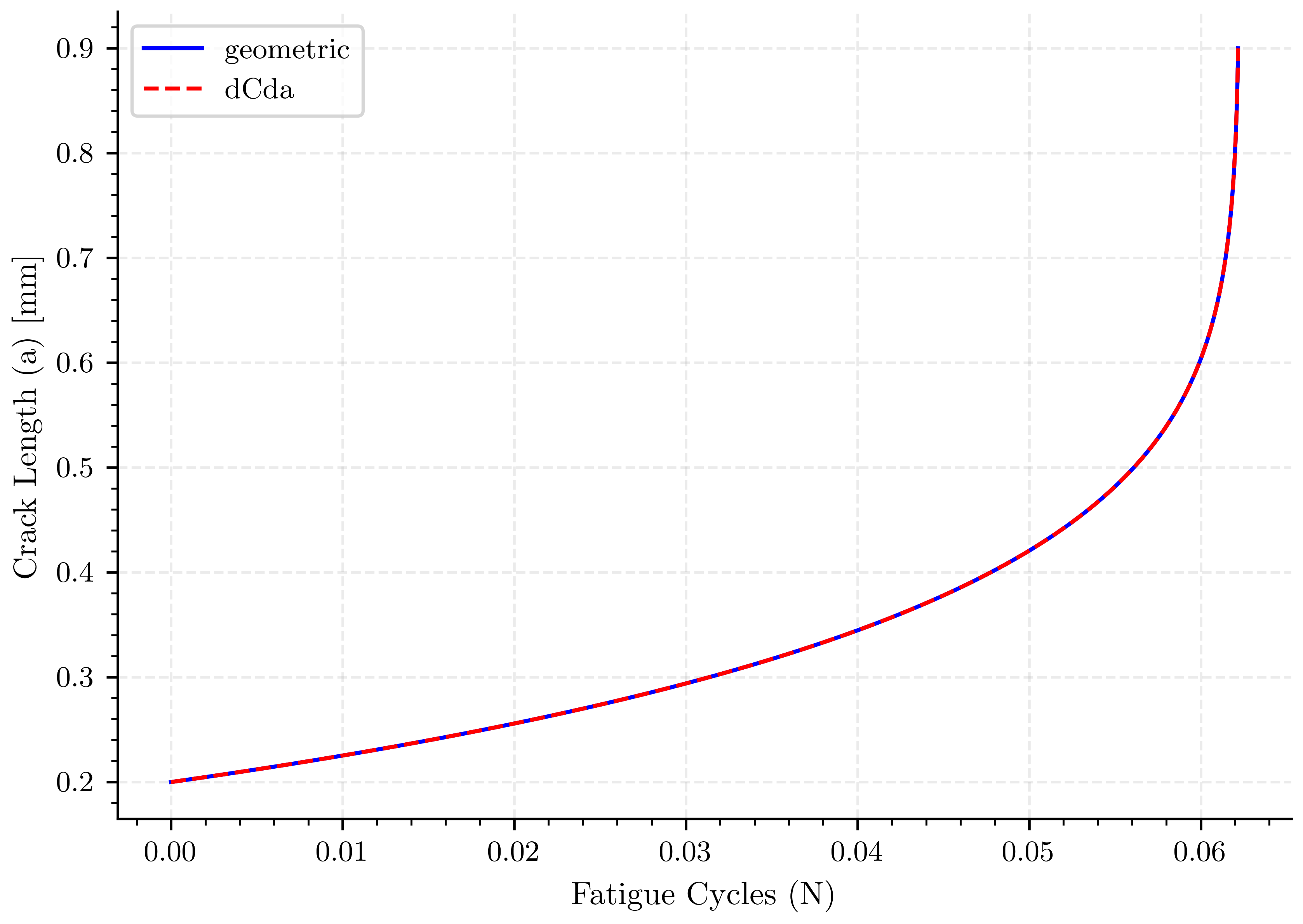
Crack area vs number of cycles#
The number of cycles to failure is calculated from the compliance respect the crack area for the different methods.
fig, ax1 = plt.subplots()

ax1.plot(Nf_f_geometric, a_fatigue, 'b-', label=r"geometric")
ax1.plot(Nf_dCda, a_fatigue, 'r--', label=r"dCda")

ax1.set_xlabel(pcfg.cycles_label)
ax1.set_ylabel(pcfg.crack_length_label)
ax1.legend()

plt.show()

header_fatigue = "cycles\ta"
results_fatigue = np.column_stack((Nf_dCda, a_fatigue))
np.savetxt(
    os.path.join(
        results_folder,
        f"a_{str(a0_fatigue).replace('.', '')}_{str(af_fatigue).replace('.', '')}.lefm_fatigue"
    ),
    results_fatigue, fmt="%.6e", delimiter="\t", header=header_fatigue, comments=""
)

plt.show()
Total running time of the script: (0 minutes 11.973 seconds)