
Note
Go to the end to download the full example code.
Simulation 6#
The model represents a square plate with a central crack, as shown in the figure below. The bottom part is fixed in all directions, while the upper part can slide vertically. A vertical displacement is applied at the top. The geometry and boundary conditions are depicted in the figure. We discretize the model with quadrilateral elements.
Note
In this case, only one quarter of the model will be considered due to symmetry. Additionally, a regular mesh will be used.
#           u/\/\/\/\/\/\       u/\/\/\/\/\/\
#            ||||||||||||        ||||||||||||
#            *----------*    o|\ *----------*
#            |          |    o|/ |          |
#            | 2a=1.0   |    o|\ | a=a0     |
#            |   ----   |    o|/ *----------*
#            |          |             /_\/_\
#            |          |            oo oo oo
#            *----------*
#            /_\/_\/_\/_\
#     |Y    /////////////
#     |
#     *---X
The Young’s modulus, Poisson’s ratio, and the critical energy release rate are given in the table Properties. Young’s modulus \(E\) and Poisson’s ratio \(\nu\) can be represented with the Lamé parameters as: \(\lambda=\frac{E\nu}{(1+\nu)(1-2\nu)}\); \(\mu=\frac{E}{2(1+\nu)}\).
VALUE |
UNITS |
|
|---|---|---|
E |
210 |
kN/mm2 |
nu |
0.3 |
[-] |
Gc |
0.0027 |
kN/mm |
l |
0.015 |
mm |
Import necessary libraries#
import numpy as np
import dolfinx
import mpi4py
import petsc4py
import os
Import from phasefieldx package#
from phasefieldx.Element.Phase_Field_Fracture.Input import Input
from phasefieldx.Element.Phase_Field_Fracture.solver.solver_ener_non_variational import solve
from phasefieldx.Boundary.boundary_conditions import bc_y, bc_x, get_ds_bound_from_marker
from phasefieldx.PostProcessing.ReferenceResult import AllResults
Parameters Definition#
Data is an input object containing essential parameters for simulation setup and result storage:
E: Young’s modulus, set to 210 \(kN/mm^2\).
nu: Poisson’s ratio, set to 0.3.
Gc: Critical energy release rate, set to 0.0027 \(kN/mm\).
l: Length scale parameter, set to 0.0025 \(mm\).
degradation: Specifies the degradation type. Options are “isotropic” or “anisotropic”.
split_energy: Controls how the energy is split; options include “no” (default), “spectral,” or “deviatoric.”
degradation_function: Specifies the degradation function; here, it is “quadratic.”
irreversibility: Not used/implemented for this solver.
save_solution_xdmf and save_solution_vtu: Specify the file formats to save displacement results. In this case, results are saved as .vtu files.
results_folder_name: Name of the folder for saving results. If it exists, it will be replaced with a new empty folder.
Data = Input(E=210.0,
             nu=0.3,
             Gc=0.0027,
             l=0.0025,
             degradation="isotropic",
             split_energy="not_applied",
             degradation_function="quadratic",
             irreversibility="not_applied",
             fatigue=False,
             fatigue_degradation_function="not_applied",
             fatigue_val=None,
             k=0.0,
             save_solution_xdmf=False,
             save_solution_vtu=True,
             results_folder_name="results_6_a07_l2")
- Mesh Definition
The mesh is a structured grid with quadrilateral elements:
divx, divy: Number of elements along the x and y axes.
lx, ly: Physical domain dimensions in x and y.
The mesh is generated using Gmsh and saved as a ‘mesh.msh’ file. For more details on how to create the mesh, refer to the ref_example_geo_gomes examples.
msh_file = os.path.join("../GmshGeoFiles/Central_cracked/central_cracked.msh")  # Path to the mesh file
# msh_file = os.path.join("mesh.msh")  # Path to the mesh file
gdim = 2                                    # Geometric dimension of the mesh
gmsh_model_rank = 0                        # Rank of the Gmsh model in a parallel setting
mesh_comm = mpi4py.MPI.COMM_WORLD            # MPI communicator for parallel computation
The mesh, cell markers, and facet markers are extracted from the ‘mesh.msh’ file using the read_from_msh function.
msh, cell_markers, facet_markers = dolfinx.io.gmshio.read_from_msh(msh_file, mesh_comm, gmsh_model_rank, gdim)

fdim = msh.topology.dim - 1 # Dimension of the mesh facets
h=0.001

# h = 1/divx
a0 = 0.7
ly = 3.0
Boundary Identification#
Boundary conditions are applied to specific regions of the domain:
bottom: Identifies the \(y=0\) and \(x>a0\) boundary.
top: Identifies the \(y=ly\) boundary.
left: Identifies the \(x=0\) boundary.
fdim is the dimension of boundary facets (1D for a 2D mesh).
def bottom(x):
    return np.logical_and(np.isclose(x[1], 0), np.greater_equal(x[0], a0))

def top(x):
    return np.isclose(x[1], ly)

def left(x):
    return np.isclose(x[0], 0.0)

fdim = msh.topology.dim - 1 # Dimension of the mesh facets
These markers are used to apply boundary conditions and external loads to specific regions of the domain:
bottom_facet_marker: Identifies the bottom boundary where y=0 and x >= a0.
top_facet_marker: Identifies the top boundary where y=ly.
left_facet_marker: Identifies the left boundary where x=0.
The locate_entities_boundary function is used to locate the facets on the mesh that satisfy the specified conditions for each boundary.
bottom_facet_marker = dolfinx.mesh.locate_entities_boundary(msh, fdim, bottom)
top_facet_marker = dolfinx.mesh.locate_entities_boundary(msh, fdim, top)
left_facet_marker = dolfinx.mesh.locate_entities_boundary(msh, fdim, left)
Selecting the top face marker as the target location where the external force will be applied during the simulation:
ds_top = get_ds_bound_from_marker(top_facet_marker, msh, fdim)

ds_list = np.array([
                   [ds_top, "top"],
                   ])
Function Space Definition#
Define function spaces for displacement and phase-field using Lagrange elements.
V_u = dolfinx.fem.functionspace(msh, ("Lagrange", 1, (msh.geometry.dim, )))
V_phi = dolfinx.fem.functionspace(msh, ("Lagrange", 1))
Boundary Conditions#
The boundary conditions are applied as follows:
The bottom nodes are constrained in the vertical direction (y), allowing horizontal movement (x displacement unconstrained).
The left nodes are constrained in the horizontal direction (x), allowing vertical movement (y displacement unconstrained).
bc_bottom = bc_y(bottom_facet_marker, V_u, fdim)
bc_left = bc_x(left_facet_marker, V_u, fdim)
The bcs_list_u variable is a list that stores all boundary conditions for the displacement field \(\boldsymbol u\). This list facilitates easy management of multiple boundary conditions and can be expanded if additional conditions are needed.
bcs_list_u = [bc_bottom,  bc_left]
bcs_list_u_names = ["bottom",  "left"]
External Load Definition#
Here, we define the external load to be applied to the top boundary (ds_top). T_top represents the external force applied in the y-direction.
surface_aplication_force = 1.0
T_top = dolfinx.fem.Constant(msh, petsc4py.PETSc.ScalarType((0.0, 1.0/surface_aplication_force)))
The load is added to the list of external loads, T_list_u, which will be updated incrementally in the update_loading function.
T_list_u = [
           [T_top, ds_top]
           ]
f = None
Boundary Conditions for phase field
bcs_list_phi = []
Solver Call for a Phase-Field Fracture Problem#
final_gamma = 0.7
Uncomment the following lines to run the solver with the specified parameters.
c1 = 1.0
c2 = 1.0

# solve(Data,
#       msh,
#       final_gamma,
#       V_u,
#       V_phi,
#       bcs_list_u,
#       bcs_list_phi,
#       f,
#       T_list_u,
#       ds_list,
#       dtau=0.0001,
#       dtau_min=1e-12,
#       dtau_max=1.0,
#       path=None,
#       bcs_list_u_names=bcs_list_u_names,
#       c1=c1,
#       c2=c2,
#       threshold_gamma_save=0.01)
Load results#
Once the simulation finishes, the results are loaded from the results folder. The AllResults class takes the folder path as an argument and stores all the results, including logs, energy, convergence, and DOF files. Note that it is possible to load results from other results folders to compare results. It is also possible to define a custom label and color to automate plot labels.
import pyvista as pv
import pandas as pd
import matplotlib.pyplot as plt
import sys
sys.path.insert(0, os.path.abspath('../../'))
plt.style.use('../../graph.mplstyle')
import plot_config as pcfg
S = AllResults(Data.results_folder_name)
S.set_label('Simulation')
S.set_color('b')
pv.start_xvfb()
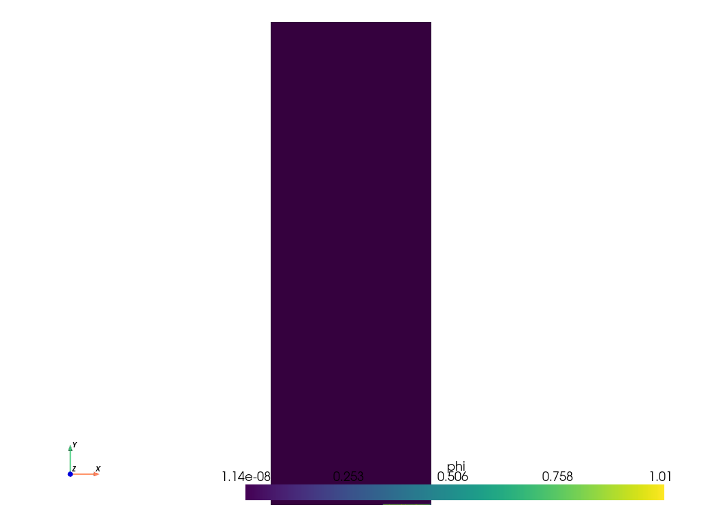
file_vtu = pv.read(os.path.join(Data.results_folder_name, "paraview-solutions_vtu", "phasefieldx_p0_000020.vtu"))
file_vtu.plot(scalars='phi', cpos='xy', show_scalar_bar=True, show_edges=False)
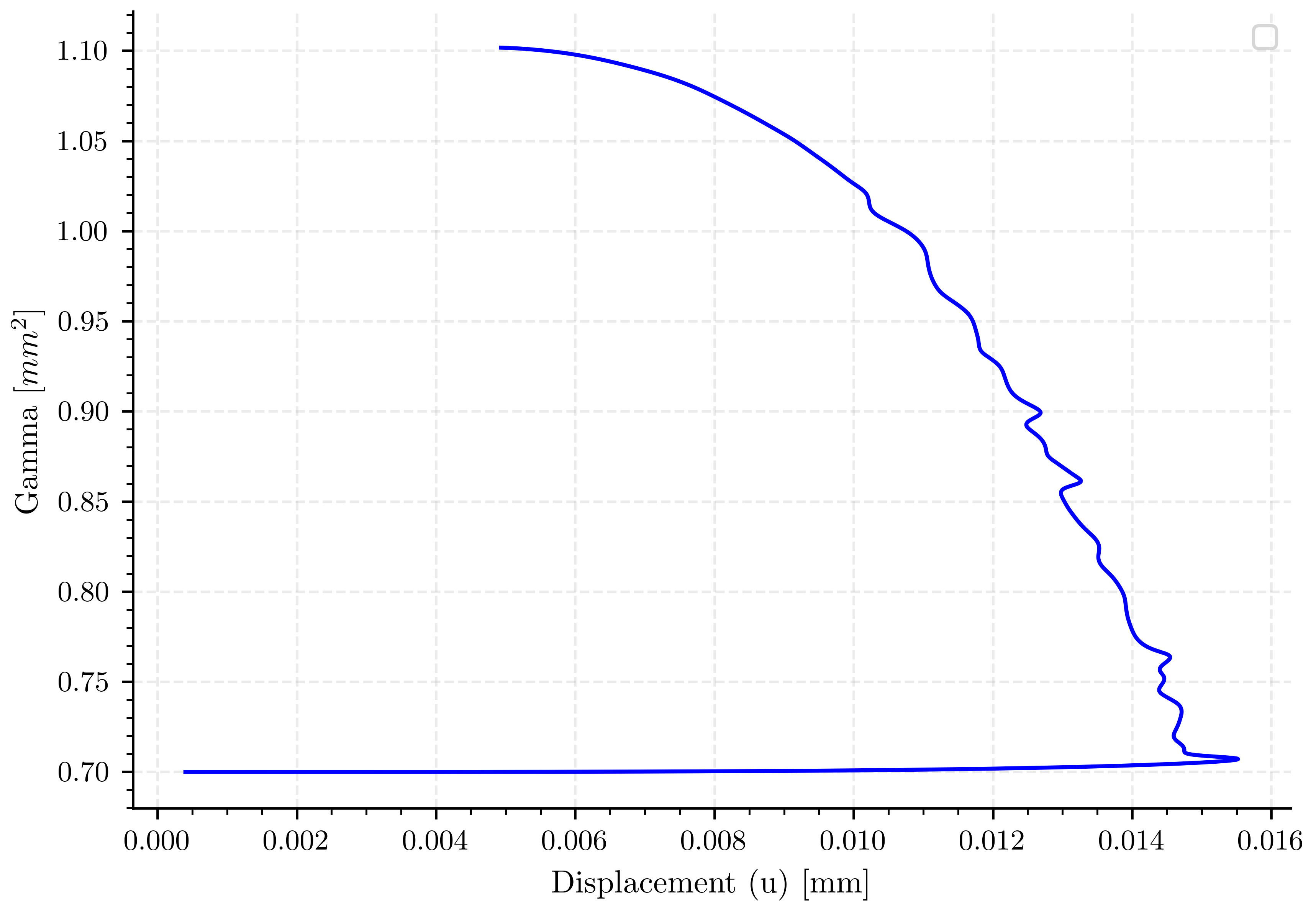
Plot: Displacement vs Fracture Energy#
force_quarter        = abs(S.reaction_files['bottom.reaction']["Ry"])
displacement_quarter = abs(2*S.energy_files['total.energy']["E"]/(S.reaction_files['bottom.reaction']["Ry"]))
stiffness_quarter    = abs(S.reaction_files['bottom.reaction']["Ry"]/displacement_quarter)
compliance_quarter   = 1/stiffness_quarter
dCda_quarter         = 2*Data.Gc/S.reaction_files['bottom.reaction']["Ry"]**2
gamma_quarter        = a0/2 + S.energy_files['total.energy']["gamma"]
lambda_quarter       = S.dof_files["lambda.dof"]["lambda"]
Complete model without corrections#
displacement_complete  = 2*displacement_quarter
force_complete         = 2*force_quarter
compliance_complete    = compliance_quarter
stiffness_complete     = stiffness_quarter
dCda_complete          = dCda_quarter/2.0
gamma_complete         = a0 + 2.0 * S.energy_files['total.energy']["gamma"]
gamma_phi_complete     = a0 + 2.0 * S.energy_files['total.energy']["gamma_phi"]
gamma_gradphi_complete = a0 + 2.0 * S.energy_files['total.energy']["gamma_gradphi"]


header = ["displacement", "force", "gamma", "compliance", "stiffness", "dCda"]
data_save = np.column_stack((displacement_complete, force_complete, gamma_complete, compliance_complete,stiffness_complete, dCda_complete))
save_path = os.path.join(Data.results_folder_name, "results.pff")
# np.savetxt(save_path, data_save, fmt="%.6e", delimiter="\t", header="\t".join(header), comments="")
Complete model with Gc corrections#
gc_factor = 1 + 2*h/(2*Data.l)
displacement_complete_corrected_gc  = displacement_complete/np.sqrt(gc_factor)
force_complete_corrected_gc         = force_complete/np.sqrt(gc_factor)
compliance_complete_corrected_gc    = compliance_complete
stiffness_complete_corrected_gc     = stiffness_complete
dCda_complete_corrected_gc          = dCda_complete*gc_factor
gamma_complete_corrected_gc         = a0 + 2.0 * S.energy_files['total.energy']["gamma"]/gc_factor
gamma_phi_complete_corrected_gc     = a0 + 2.0 * S.energy_files['total.energy']["gamma_phi"]/gc_factor
gamma_gradphi_complete_corrected_gc = a0 + 2.0 * S.energy_files['total.energy']["gamma_gradphi"]/gc_factor


header = ["displacement", "force", "gamma", "compliance", "stiffness", "dCda", "lambda"]
data_save = np.column_stack((displacement_complete_corrected_gc, force_complete_corrected_gc, gamma_complete_corrected_gc, compliance_complete_corrected_gc,stiffness_complete_corrected_gc, dCda_complete_corrected_gc))
save_path = os.path.join(Data.results_folder_name, "results_corrected_bourdin.pff")
# np.savetxt(save_path, data_save, fmt="%.6e", delimiter="\t", header="\t".join(header), comments="")
Plot: Force vs Vertical Displacement#
fig, energyg = plt.subplots()

energyg.plot(displacement_complete, gamma_complete, 'b-')

energyg.set_xlabel(pcfg.displacement_label)
energyg.set_ylabel(pcfg.gamma_label)
energyg.legend()
/home/docs/checkouts/readthedocs.org/user_builds/phasefieldfatigue/checkouts/stable/examples/Phase_Field_Central_Cracked/plot_simulation_6_a07_l2.py:332: UserWarning: No artists with labels found to put in legend.  Note that artists whose label start with an underscore are ignored when legend() is called with no argument.
  energyg.legend()

<matplotlib.legend.Legend object at 0x734c56ce2290>
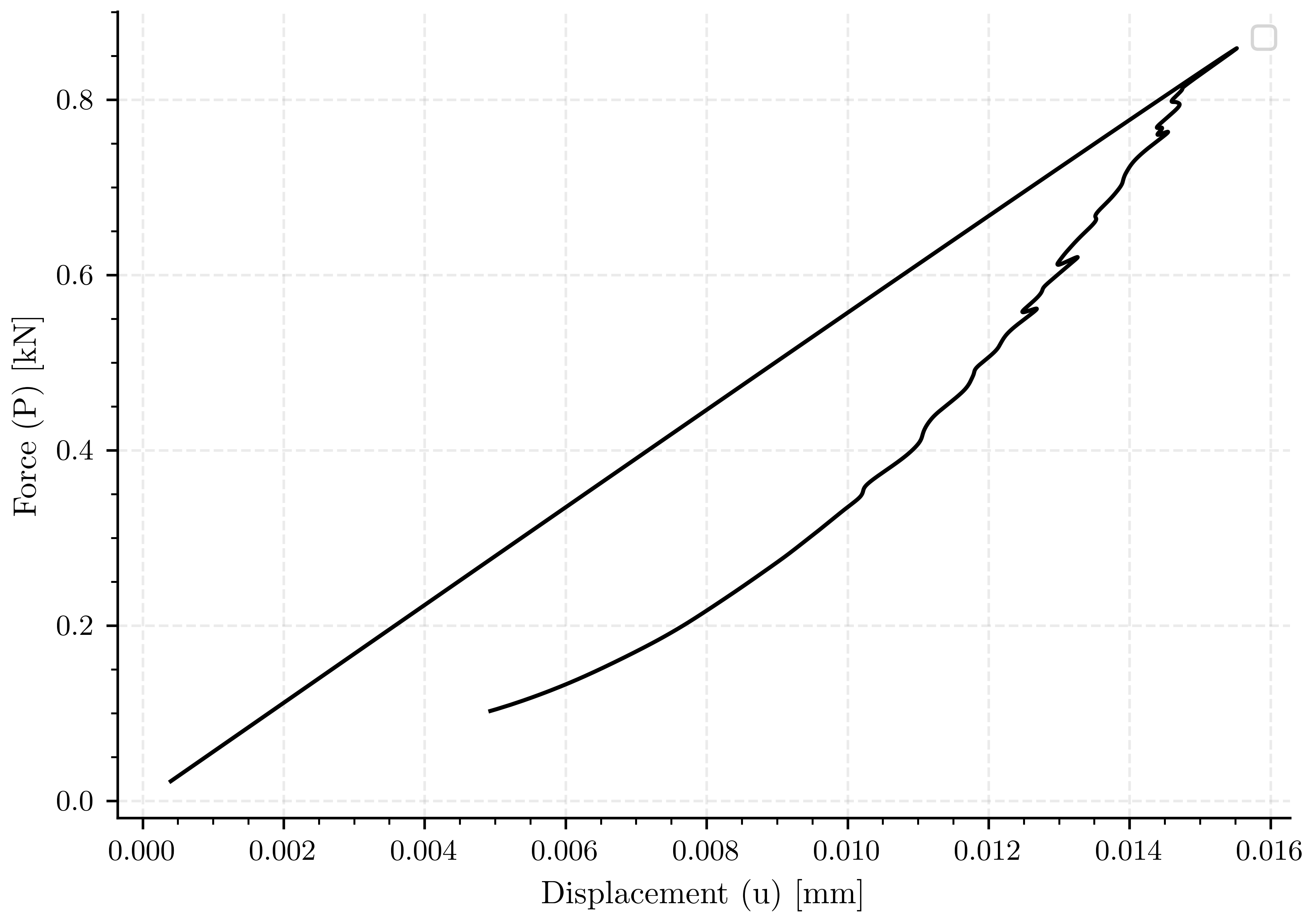
Plot: Force vs Vertical Displacement#
fig, ax_reaction = plt.subplots()

ax_reaction.plot(displacement_complete, force_complete, 'k-')

ax_reaction.set_xlabel(pcfg.displacement_label)
ax_reaction.set_ylabel(pcfg.force_label)
ax_reaction.legend()
/home/docs/checkouts/readthedocs.org/user_builds/phasefieldfatigue/checkouts/stable/examples/Phase_Field_Central_Cracked/plot_simulation_6_a07_l2.py:344: UserWarning: No artists with labels found to put in legend.  Note that artists whose label start with an underscore are ignored when legend() is called with no argument.
  ax_reaction.legend()

<matplotlib.legend.Legend object at 0x734c56cefee0>
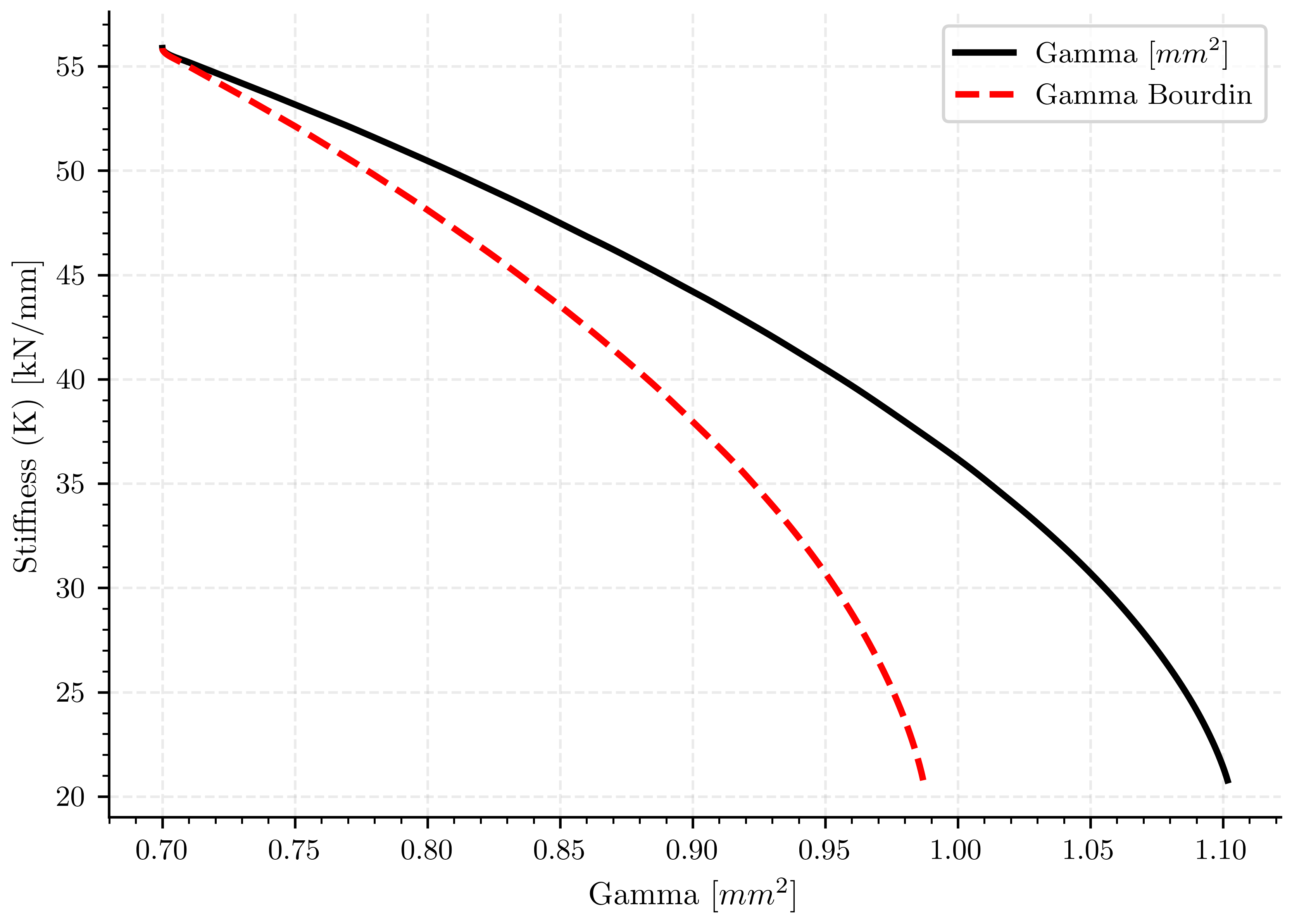
Plot: Force vs Vertical Displacement#
fig, ax_reaction = plt.subplots()

ax_reaction.plot(gamma_complete, stiffness_complete, 'k-', linewidth=2.0, label=pcfg.gamma_label)
ax_reaction.plot(gamma_complete_corrected_gc, stiffness_complete, 'r--', linewidth=2.0, label=pcfg.gamma_bourdin_label)

ax_reaction.set_xlabel(pcfg.gamma_label)
ax_reaction.set_ylabel(pcfg.stiffness_label)
ax_reaction.legend()

plt.show()
Total running time of the script: (0 minutes 7.838 seconds)