Note
Go to the end to download the full example code.
Specimen 2#
This example demonstrates the simulation of a compact specimen with a phase-field fracture model. The specimen geometry corresponds to a configuration where the parameter \(H\) is set to 1.6 mm.
The mesh used for this simulation is generated using Gmsh and is based on the geometry described in Specimen 2. This geometry includes predefined regions and boundary markers essential for applying boundary conditions and loads during the simulation.
Import necessary libraries#
import numpy as np
import dolfinx
import mpi4py
import petsc4py
import os
Import from phasefieldx package#
from phasefieldx.Element.Phase_Field_Fracture.Input import Input
from phasefieldx.Element.Phase_Field_Fracture.solver.solver_ener_non_variational import solve
from phasefieldx.Boundary.boundary_conditions import bc_xy, get_ds_bound_from_marker
from phasefieldx.PostProcessing.ReferenceResult import AllResults
Parameters Definition#
Data is an input object containing essential parameters for simulation setup and result storage:
E: Young’s modulus, set to 211 \(kN/mm^2\).
nu: Poisson’s ratio, set to 0.3.
Gc: Critical energy release rate, set to 0.0073 \(kN/mm\).
l: Length scale parameter, set to 0.1 \(mm\).
degradation: Specifies the degradation type. Options are “isotropic” or “anisotropic”.
split_energy: Controls how the energy is split; options include “no” (default), “spectral,” or “deviatoric.”
degradation_function: Specifies the degradation function; here, it is “quadratic.”
irreversibility: Not used/implemented for this solver.
save_solution_xdmf and save_solution_vtu: Specify the file formats to save displacement results. In this case, results are saved as .vtu files.
results_folder_name: Name of the folder for saving results. If it exists, it will be replaced with a new empty folder.
Data = Input(E=211.0,   # young modulus
             nu=0.3,    # poisson
             Gc=0.073,  # critical energy release rate
             l=0.1,     # lenght scale parameter
             degradation="isotropic",  # "isotropic" "anisotropic"
             split_energy="no",       # "spectral" "deviatoric"
             degradation_function="quadratic",
             irreversibility="no",  # "miehe"
             fatigue=False,
             fatigue_degradation_function="no",
             fatigue_val=0.0,
             k=0.0,
             save_solution_xdmf=False,
             save_solution_vtu=True,
             results_folder_name="results_specimen_2_H16")

b = 40.0
a0 = 0.2*b
Mesh Importation#
The mesh is generated using Gmsh and saved in the ‘.msh’ format. For this example, the mesh is based on the geometry defined in the .geo file, which is provided in the reference example_geo_specimen_2_H16.
msh_file = os.path.join("../GmshGeoFiles/Compact_specimen/specimen_2_H16.msh")  # Path to the mesh file
gdim = 2                           # Geometric dimension of the mesh
gmsh_model_rank = 0                # Rank of the Gmsh model in a parallel setting
mesh_comm = mpi4py.MPI.COMM_WORLD  # MPI communicator for parallel computation
The mesh, cell markers, and facet markers are extracted from the ‘mesh.msh’ file using the read_from_msh function.
msh, cell_markers, facet_markers = dolfinx.io.gmshio.read_from_msh(msh_file, mesh_comm, gmsh_model_rank, gdim)
fdim = msh.topology.dim - 1 # Dimension of the mesh facets
The mesh size along the expected crack propagation path is defined as follows: Here, h represents the characteristic element size in the region of interest.
b = 40.0  # Characteristic dimension of the specimen
h = 0.001 * b  # Element size scaled by the specimen's characteristic dimension
Facets defined in the .geo file used to generate the ‘.msh’ file are identified here. Each marker variable corresponds to a specific region on the specimen:
top_top_facet_marker: Refers to the top part of the top circle of the specimen.
top_bottom_facet_marker: Refers to the bottom part of the top circle of the specimen.
bottom_top_facet_marker: Refers to the top part of the bottom circle of the specimen.
bottom_bottom_facet_marker: Refers to the bottom part of the bottom circle of the specimen.
top_top_facet_marker = facet_markers.find(204)
top_bottom_facet_marker = facet_markers.find(205)
bottom_top_facet_marker = facet_markers.find(206)
bottom_bottom_facet_marker = facet_markers.find(203)
Using the bottom and top functions, we locate the facets on the top part of the top circle of the mesh, where the force will be applied. The locate_entities_boundary function returns an array of facet indices representing these identified boundary entities.
ds_top = get_ds_bound_from_marker(top_top_facet_marker, msh, fdim)

ds_list = np.array([
                   [ds_top, "top"],
                   ])
Function Space Definition#
Define function spaces for displacement and phase-field.
V_u = dolfinx.fem.functionspace(msh, ("Lagrange", 1, (msh.geometry.dim, )))
V_phi = dolfinx.fem.functionspace(msh, ("Lagrange", 1))
The boundary condition is applied to the bottom part of the bottom circle of the specimen. This boundary condition fixes the displacement in all directions, ensuring that this part of the specimen remains stationary during the simulation.
bc_bottom_bottom = bc_xy(bottom_bottom_facet_marker, V_u, fdim)

# The list of Dirichlet boundary conditions for the displacement field is defined here.
# Currently, it includes only the boundary condition applied to the bottom part of the bottom circle.
bcs_list_u = [bc_bottom_bottom]

# A corresponding list of names for the boundary conditions is also defined for easier identification.
bcs_list_u_names = ["bottom_bottom"]
External Load Definition#
Here, we define the external load to be applied to the top boundary (ds_top). T_top represents the external force applied in the y-direction.
surface_aplication_force = np.pi*0.25*40.0/2.0
T_top = dolfinx.fem.Constant(msh, petsc4py.PETSc.ScalarType((0.0, 1.0/surface_aplication_force)))
The load is added to the list of external loads, T_list_u, which will be updated incrementally in the update_loading function.
T_list_u = [
           [T_top, ds_top]
           ]
f = None
Boundary Conditions for phase field
bcs_list_phi = []
Solver Call for a Phase-Field Fracture Problem#
This section sets up and calls the solver for a phase-field fracture problem.
Key Points:
The simulation is run for a final time of 200, with a time step of 1.0.
The solver will manage the mesh, boundary conditions, and update the solution over the specified time steps.
Parameters:
dt: The time step for the simulation, set to 1.0.
final_time: The total simulation time, set to 200.0, which determines how long the problem will be solved.
path: Optional parameter for specifying the folder where results will be saved; here it is set to None, meaning results will be saved to the default location.
Function Call: The solve function is invoked with the following arguments:
Data: Contains the simulation parameters and configurations.
msh: The mesh representing the domain for the problem.
final_time: The total duration of the simulation (200.0).
V_u: Function space for the displacement field, \(\boldsymbol{u}\).
V_phi: Function space for the phase field, \(\phi\).
bcs_list_u: List of Dirichlet boundary conditions for the displacement field.
bcs_list_phi: List of boundary conditions for the phase field (empty in this case).
update_boundary_conditions: Function to update boundary conditions for the displacement field.
f: The body force applied to the domain (if any).
T_list_u: Time-dependent loading parameters for the displacement field.
update_loading: Function to update loading parameters for the quasi-static analysis.
ds_list: Boundary measures for integration over the domain boundaries.
dt: The time step for the simulation.
path: Directory for saving results (if specified).
This setup provides a framework for solving static problems with specified boundary conditions and loading parameters.
final_gamma = 200.0
Uncomment the following lines to run the solver with the specified parameters.
c1 = 1.0
c2 = 1.0

# solve(Data,
#       msh,
#       final_gamma,
#       V_u,
#       V_phi,
#       bcs_list_u,
#       bcs_list_phi,
#       f,
#       T_list_u,
#       ds_list,
#       dtau=0.0001,
#       dtau_min=1e-12,
#       dtau_max=1.0,
#       path=None,
#       bcs_list_u_names=bcs_list_u_names,
#       c1=c1,
#       c2=c2,
#       threshold_gamma_save=0.1)


import pyvista as pv
import pandas as pd
import matplotlib.pyplot as plt
import sys
sys.path.insert(0, os.path.abspath('../../'))
plt.style.use('../../graph.mplstyle')
import plot_config as pcfg
Load results#
Once the simulation finishes, the results are loaded from the results folder. The AllResults class takes the folder path as an argument and stores all the results, including logs, energy, convergence, and DOF files.
S = AllResults(Data.results_folder_name)
S.set_label('Simulation')
S.set_color('b')

# Specimen geometry parameters
b = 40.0    # Specimen width
a0 = 0.2*b  # Initial crack length
Complete model without corrections#
displacement  = abs(2*S.energy_files['total.energy']["E"]/(S.reaction_files['bottom_bottom.reaction']["Ry"]))
force         = abs(S.reaction_files['bottom_bottom.reaction']["Ry"])
stiffness     = abs(S.reaction_files['bottom_bottom.reaction']["Ry"]/displacement)
compliance    = 1/stiffness
dCda         = 2*Data.Gc/S.reaction_files['bottom_bottom.reaction']["Ry"]**2
gamma         = a0 + S.energy_files['total.energy']["gamma"]
gamma_phi     = a0/2 +  S.energy_files['total.energy']["gamma_phi"]
gamma_gradphi = a0/2 +  S.energy_files['total.energy']["gamma_gradphi"]


header = ["displacement", "force", "gamma", "compliance", "stiffness", "dCda"]
data_save = np.column_stack((displacement, force, gamma, compliance, stiffness, dCda))
save_path = os.path.join(Data.results_folder_name, "results.pff")
# np.savetxt(save_path, data_save, fmt="%.6e", delimiter="\t", header="\t".join(header), comments="")
Complete model with Gc corrections#
# Extract and compute key quantities from simulation result

# Corrections for finite element discretization effects
gc_factor = 1 + h/(2*Data.l)
displacement_corrected_gc  = displacement/np.sqrt(gc_factor)
force_corrected_gc         = force/np.sqrt(gc_factor)
compliance_corrected_gc    = compliance
stiffness_corrected_gc     = stiffness
dCda_corrected_gc          = dCda*gc_factor
gamma_corrected_gc         = a0 + S.energy_files['total.energy']["gamma"]/gc_factor
gamma_phi_corrected_gc     = a0/2 + S.energy_files['total.energy']["gamma_phi"]/gc_factor
gamma_gradphi_corrected_gc = a0/2 + S.energy_files['total.energy']["gamma_gradphi"]/gc_factor


header = ["displacement", "force", "gamma", "compliance", "stiffness", "dCda", "lambda"]
data_save = np.column_stack((displacement_corrected_gc, force_corrected_gc, gamma_corrected_gc, compliance_corrected_gc, stiffness_corrected_gc, dCda_corrected_gc))
save_path = os.path.join(Data.results_folder_name, "results_corrected_bourdin.pff")
# np.savetxt(save_path, data_save, fmt="%.6e", delimiter="\t", header="\t".join(header), comments="")
Complete model with Geometry correction#
measure=True
if measure:
    # results_a_measured = np.loadtxt(os.path.join(Data.results_folder_name, "crack_measurement/step_time_crack_length_interpolate.txt"), skiprows=1)
    results_a_measured = np.loadtxt("../Phase_Field_Compact_Specimen/results_specimen_2_H16/crack_measurement/interpolated_step_time_crack_length.txt", skiprows=1)
    crack_measured = results_a_measured[:,1]
    geo_factor = S.energy_files['total.energy']["gamma"][0:len(crack_measured)]/crack_measured


    displacement_corrected_geo  = displacement[0:len(crack_measured)]/np.sqrt(geo_factor)
    force_corrected_geo         = force[0:len(crack_measured)]/np.sqrt(geo_factor)
    compliance_corrected_geo    = compliance[0:len(crack_measured)]
    stiffness_corrected_geo     = stiffness[0:len(crack_measured)]
    dCda_corrected_geo          = dCda[0:len(crack_measured)]*geo_factor
    gamma_corrected_geo         = a0 + S.energy_files['total.energy']["gamma"][0:len(crack_measured)]/geo_factor
    gamma_phi_corrected_geo     = a0/2 + S.energy_files['total.energy']["gamma_phi"][0:len(crack_measured)]/geo_factor
    gamma_gradphi_corrected_geo = a0/2 + S.energy_files['total.energy']["gamma_gradphi"][0:len(crack_measured)]/geo_factor


    header = ["displacement", "force", "gamma", "compliance", "stiffness", "dCda", "lambda"]
    data_save = np.column_stack((displacement_corrected_geo, force_corrected_geo, gamma_corrected_geo, compliance_corrected_geo,stiffness_corrected_geo, dCda_corrected_geo))
    save_path = os.path.join(Data.results_folder_name, "results_corrected_geometry.pff")
    # np.savetxt(save_path, data_save, fmt="%.6e", delimiter="\t", header="\t".join(header), comments="")
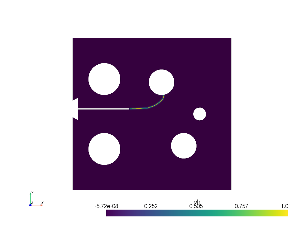
Plot: Phase-Field Distribution at Final State#
This plot visualizes the phase-field variable φ across the specimen at the final simulation step. The phase-field φ varies from 0 (intact material) to 1 (fully damaged/cracked material), showing the crack path and damage evolution.
pv.start_xvfb()
file_vtu = pv.read(os.path.join(Data.results_folder_name, "paraview-solutions_vtu", "phasefieldx_p0_000159.vtu"))
file_vtu.plot(scalars='phi', cpos='xy', show_scalar_bar=True, show_edges=False)
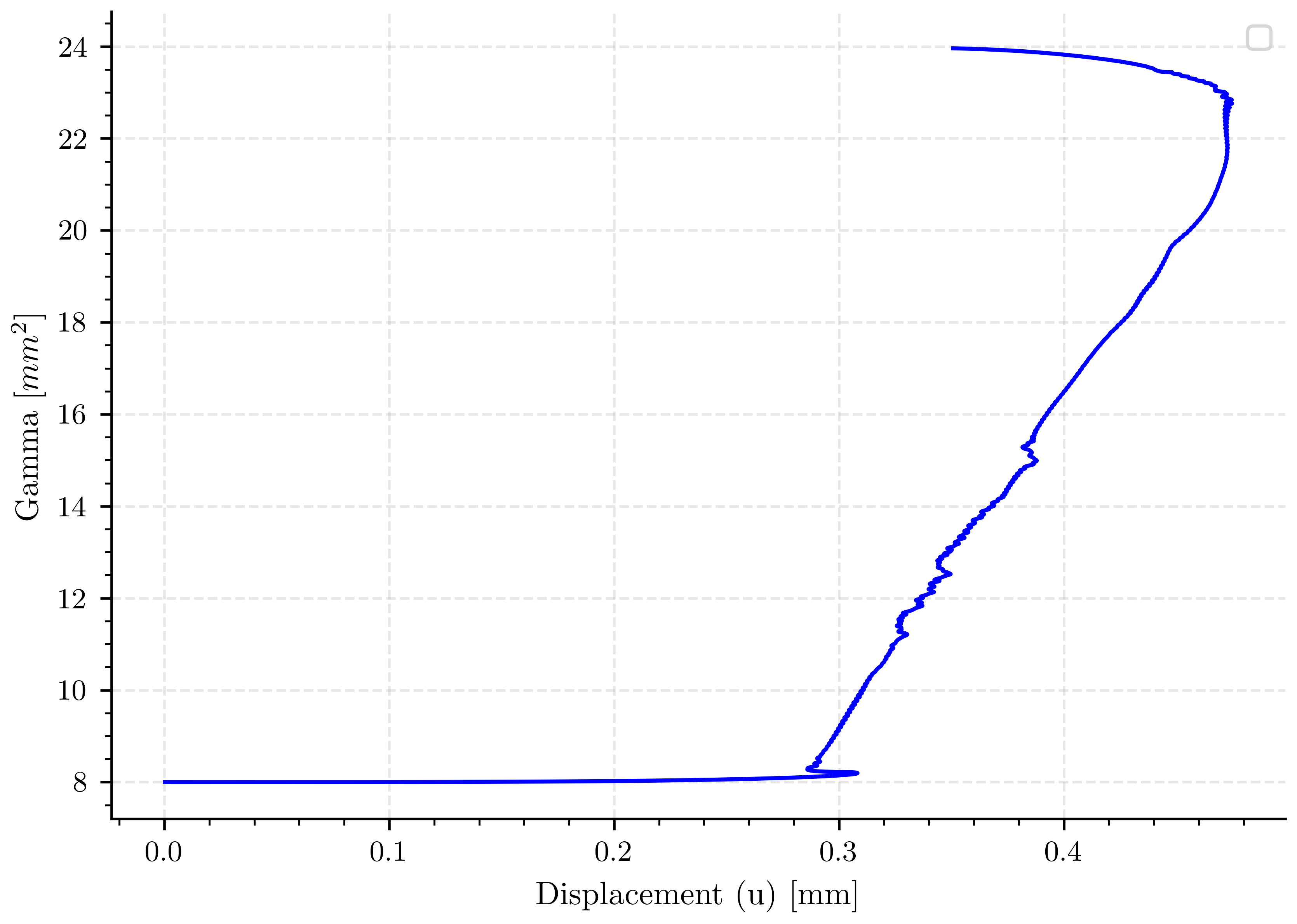
Plot: Energy Components vs Displacement#
This plot shows the evolution of different energy components during crack propagation: - γ: Total fracture energy (sum of both components below) - γ_φ: Energy contribution from the phase-field variable φ - γ_∇φ: Energy contribution from the gradient of φ (crack regularization) The displacement represents the applied loading level.
fig, ax_energy = plt.subplots()

ax_energy.plot(displacement, gamma, 'b-')

ax_energy.set_xlabel(pcfg.displacement_label)
ax_energy.set_ylabel(pcfg.gamma_label)
ax_energy.legend()
ax_energy.grid(True, alpha=0.3)
/home/docs/checkouts/readthedocs.org/user_builds/phasefieldfatigue/checkouts/stable/examples/Phase_Field_Compact_Specimen/plot_specimen_2_H16.py:345: UserWarning: No artists with labels found to put in legend.  Note that artists whose label start with an underscore are ignored when legend() is called with no argument.
  ax_energy.legend()
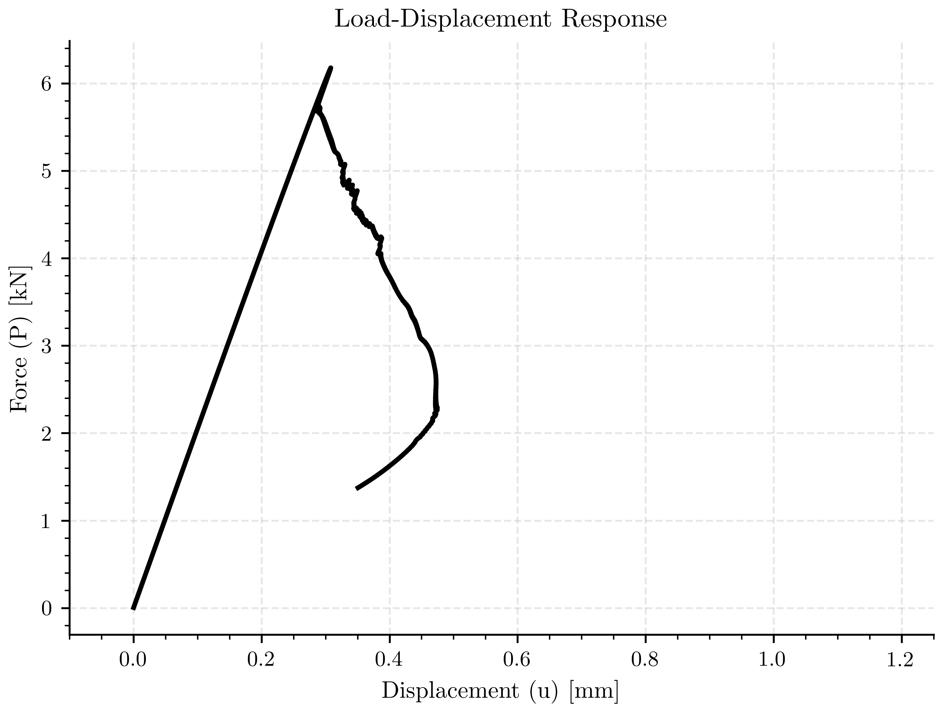
Plot: Load-Displacement Curve#
This fundamental plot shows the relationship between applied force and resulting displacement. It demonstrates the structural response including: - Initial linear elastic behavior - Peak load at crack initiation - Softening behavior during crack propagation
fig, ax_load_displacement = plt.subplots()

ax_load_displacement.plot(displacement, force, color=pcfg.color_black, linewidth=2.0)

ax_load_displacement.set_xlabel(pcfg.displacement_label)
ax_load_displacement.set_ylabel(pcfg.force_label)
ax_load_displacement.set_title('Load-Displacement Response')
ax_load_displacement.set_xlim([-0.1, 1.25])
ax_load_displacement.grid(True, alpha=0.3)
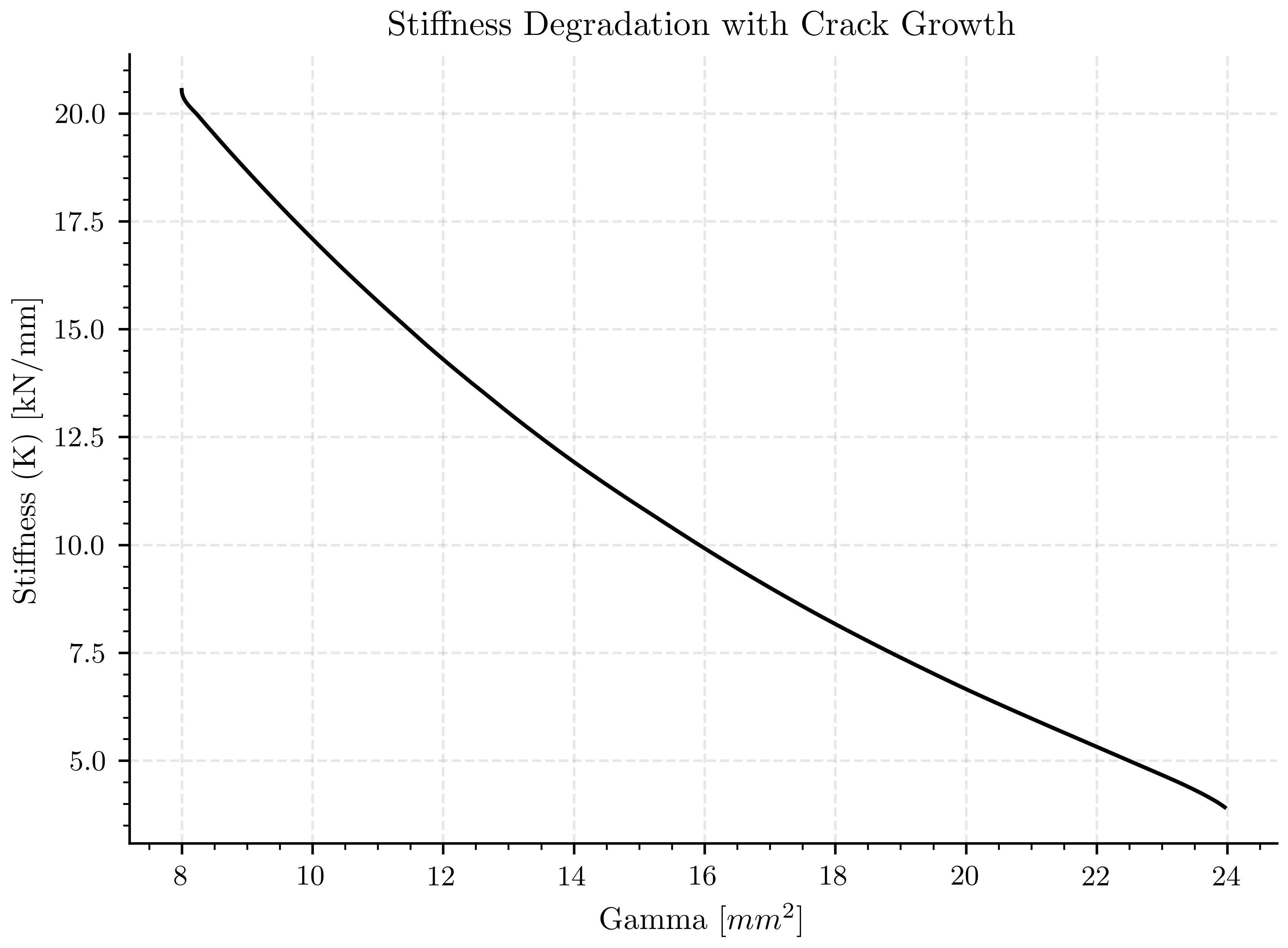
Plot: Structural Stiffness vs Crack Length#
This plot shows how the structural stiffness degrades as the crack propagates (represented by γ). Stiffness reduction is a key indicator of structural damage and is used in fracture mechanics to assess structural integrity.
fig, ax_stiffness = plt.subplots()

ax_stiffness.plot(gamma, stiffness, color=pcfg.color_black)

ax_stiffness.set_xlabel(pcfg.gamma_label)
ax_stiffness.set_ylabel(pcfg.stiffness_label)
ax_stiffness.set_title('Stiffness Degradation with Crack Growth')
ax_stiffness.grid(True, alpha=0.3)
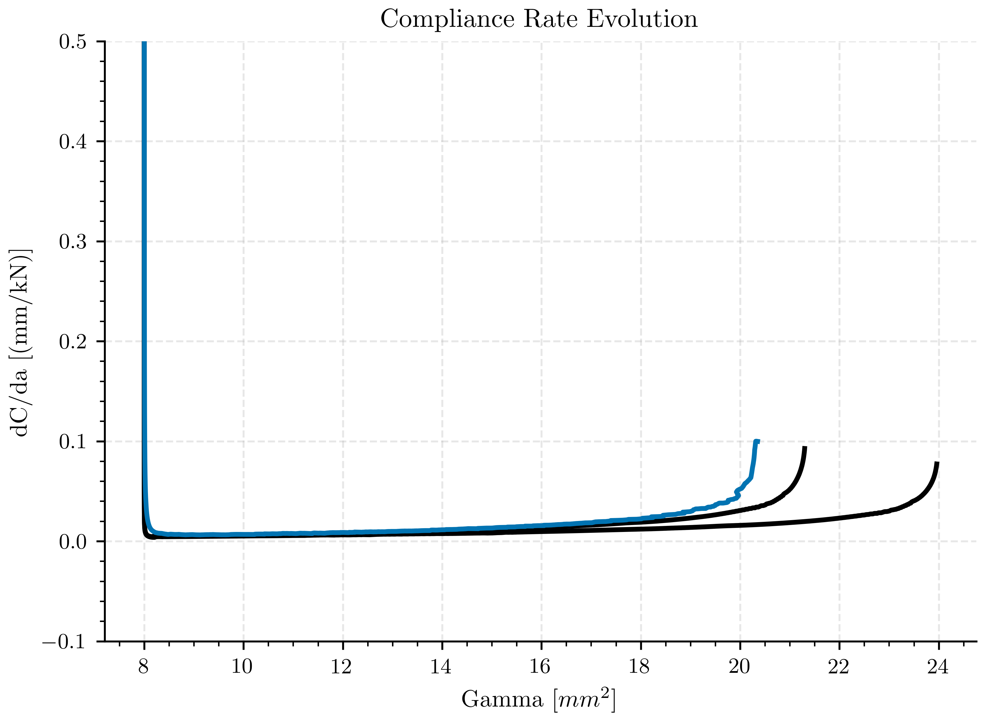
Plot: Compliance Rate vs Crack Length#
This plot displays dC/da (derivative of compliance with respect to crack length), which is a fundamental quantity in fracture mechanics. It’s directly related to the energy release rate and is used to determine crack driving forces.
fig, ax_compliance_rate = plt.subplots()

ax_compliance_rate.plot(gamma, dCda, color=pcfg.color_black, linewidth=2.0)
ax_compliance_rate.plot(gamma_corrected_gc, dCda_corrected_gc, color=pcfg.color_black, linewidth=2.0)
ax_compliance_rate.plot(gamma_corrected_geo, dCda_corrected_geo, color=pcfg.color_blue, linewidth=2.0)

ax_compliance_rate.set_xlabel(pcfg.gamma_label)
ax_compliance_rate.set_ylabel(pcfg.dCda_label)
ax_compliance_rate.set_title('Compliance Rate Evolution')
ax_compliance_rate.set_ylim([-0.1, 0.5])
ax_compliance_rate.grid(True, alpha=0.3)
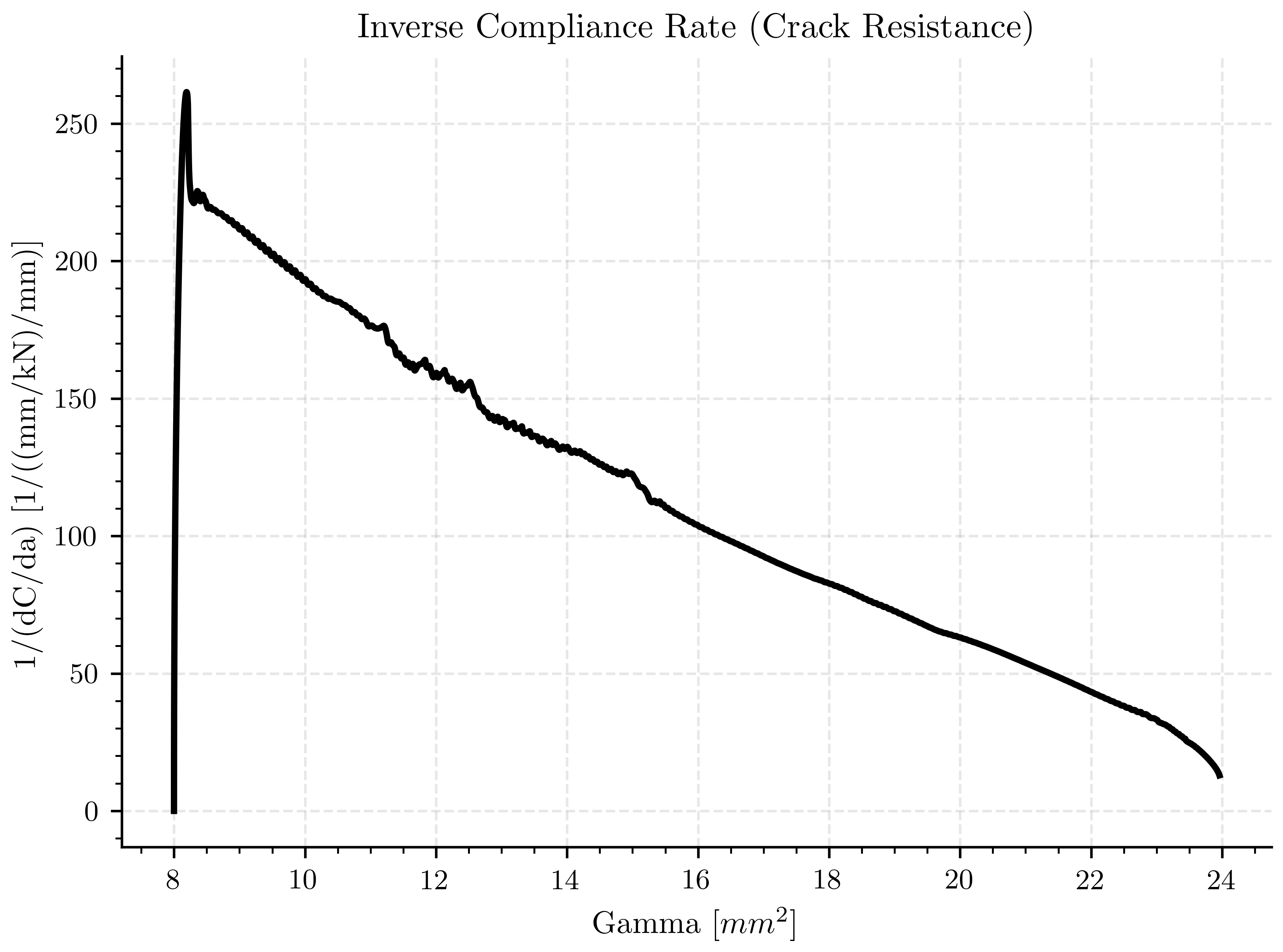
Plot: Inverse Compliance Rate vs Crack Length#
This plot shows the inverse of dC/da, which can provide insights into the crack resistance behavior. Higher values indicate greater resistance to crack propagation at that particular crack length.
fig, ax_inverse_compliance = plt.subplots()

ax_inverse_compliance.plot(gamma, 1/dCda, color=pcfg.color_black, linewidth=2.0)

ax_inverse_compliance.set_xlabel(pcfg.gamma_label)
ax_inverse_compliance.set_ylabel(pcfg.dCda_1_label)
ax_inverse_compliance.set_title('Inverse Compliance Rate (Crack Resistance)')
ax_inverse_compliance.grid(True, alpha=0.3)

plt.show()
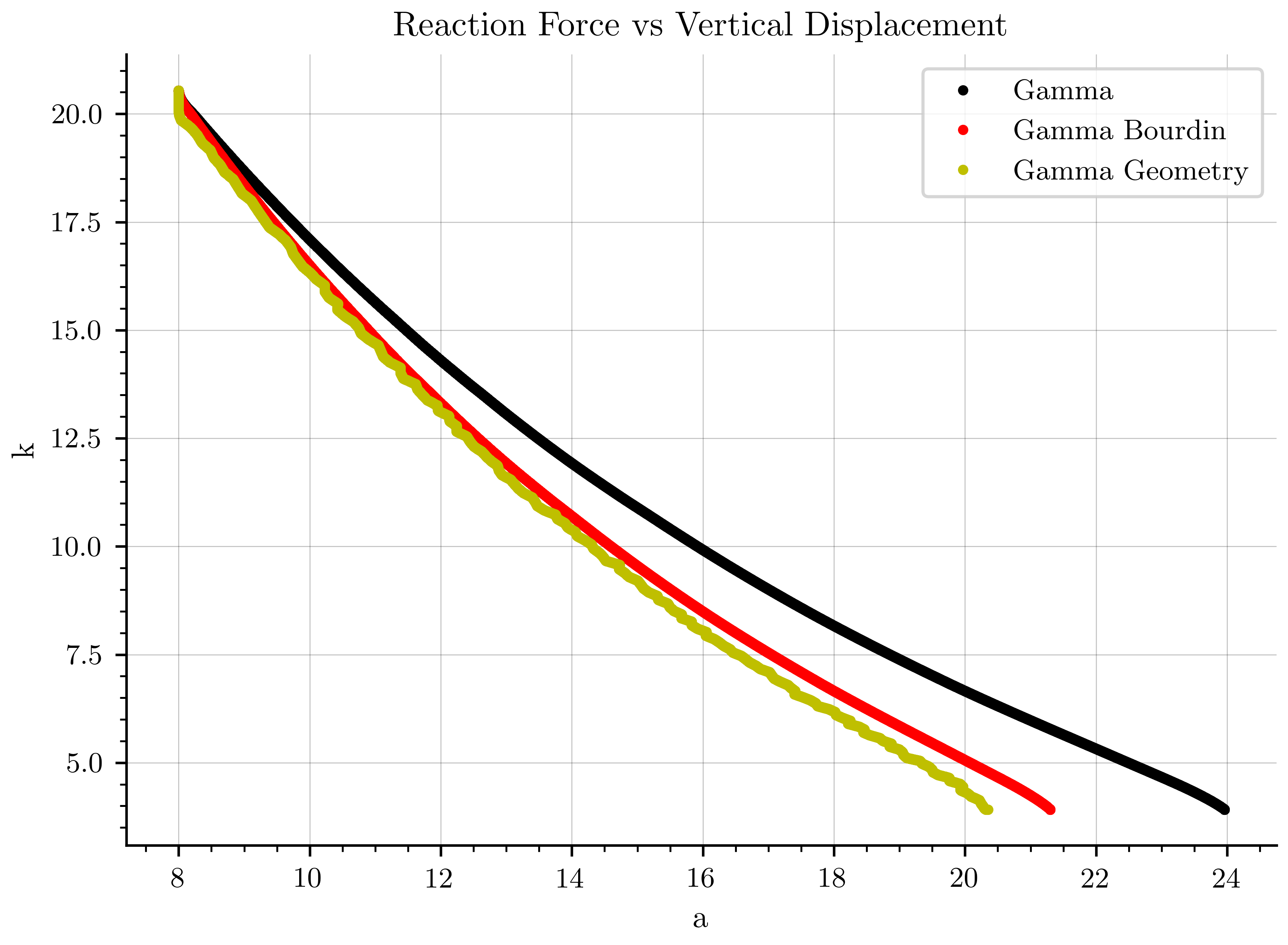
Plot: Force vs Vertical Displacement#
fig, ax_reaction = plt.subplots()

ax_reaction.plot(gamma, stiffness, 'k.', linewidth=2.0, label=pcfg.gamma_ref_label)
ax_reaction.plot(gamma_corrected_gc, stiffness, 'r.', linewidth=2.0, label=pcfg.gamma_bourdin_label)
ax_reaction.plot(gamma_corrected_geo, stiffness[0:len(gamma_corrected_geo)], 'y.', linewidth=2.0, label=pcfg.gamma_geometry_label)

ax_reaction.grid(color='k', linestyle='-', linewidth=0.3)
ax_reaction.set_xlabel('a')
ax_reaction.set_ylabel('k')
ax_reaction.set_title('Reaction Force vs Vertical Displacement')
ax_reaction.legend()
plt.show()
Load Processed Results for Further Analysis#
Load the saved processed data as a pandas DataFrame for additional analysis or external use. This provides easy access to all computed quantities. data = pd.read_csv(save_path, delimiter=”t”, comment=”#”, header=0) print(“Available data columns:”, data.columns.tolist()) print(f”Data shape: {data.shape}”) Example access: data[“gamma”], data[“force”], data[“displacement”], etc.
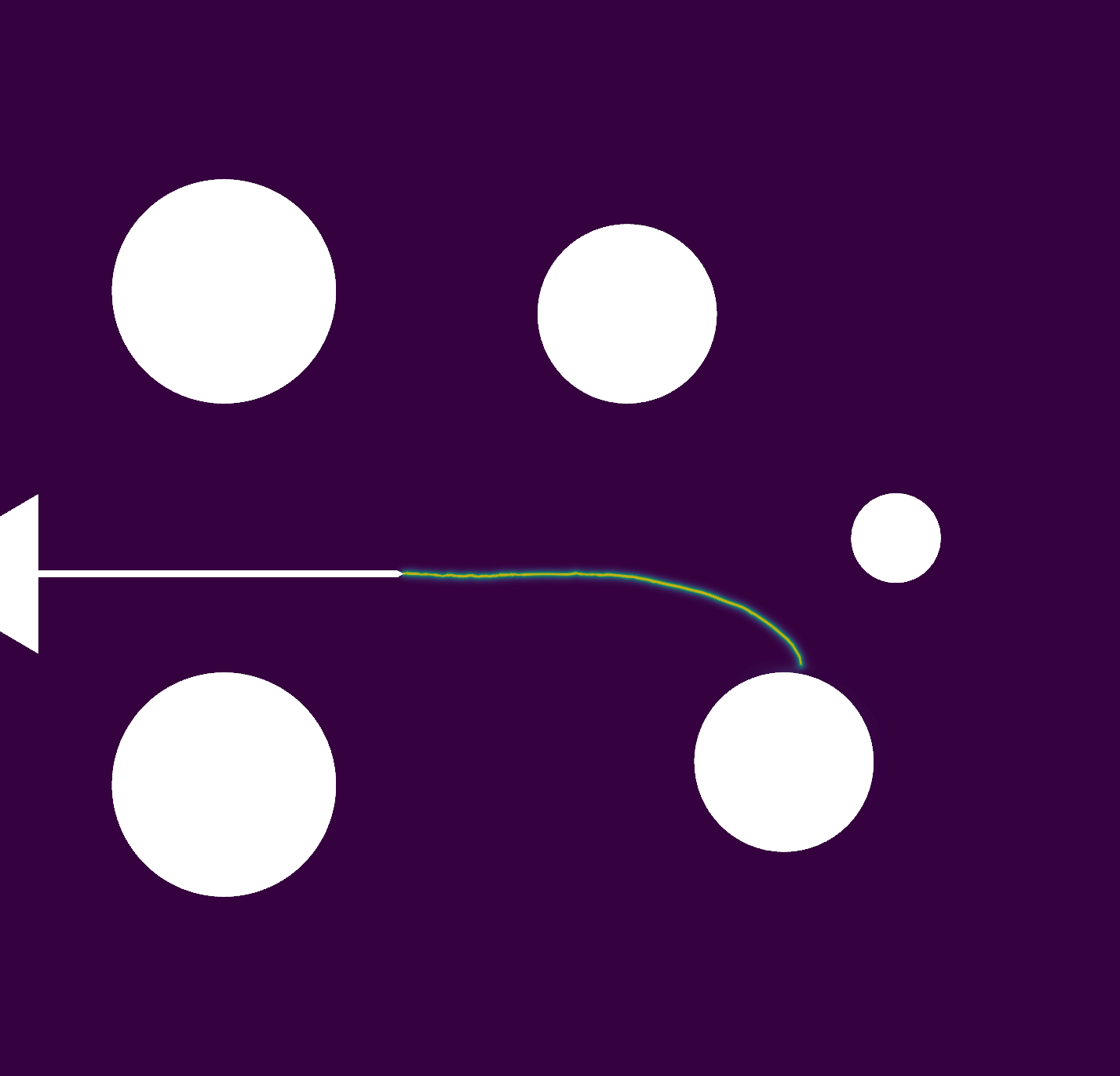
Plot: Phase-Field with Crack Path Visualization#
This 3D visualization combines the phase-field distribution with a theoretical crack path line (red line) to compare the predicted crack trajectory with the phase-field simulation results.
save_image=False
# Create a PyVista plotter
if save_image:
    # Save high-quality image of phase-field for documentation
    plotter_save = pv.Plotter(off_screen=True)
    plotter_save.add_mesh(file_vtu, scalars='phi')
    plotter_save.view_xy()
    plotter_save.remove_scalar_bar()
    plotter_save.set_background('white')
    plotter_save.camera.tight(padding=0.0)
    plotter_save.camera.clipping_range = (0.1, 1000.0)
    plotter_save.window_size = (500, 480)
    plotter_save.screenshot(os.path.join(Data.results_folder_name,'paraview_phi'),
                        transparent_background=False,
                        return_img=False)
    plotter_save.close()
Total running time of the script: (0 minutes 8.660 seconds)