
Note
Go to the end to download the full example code.
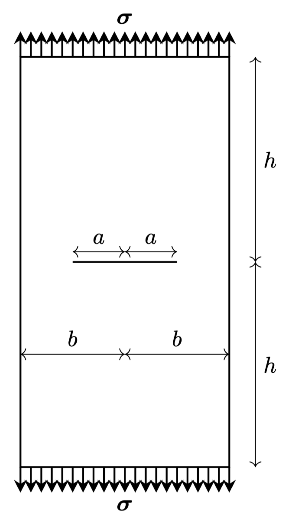
LEFM: Center-Cracked Specimen#
This script analyzes a center-cracked test specimen using Linear Elastic Fracture Mechanics (LEFM) theory. It performs:
Calculation of the stress intensity factor (\(K_I\)) based on specimen geometry and material properties.
Evaluation of the critical force (\(P_c\)) as functions of crack length (\(a\)).
Numerical integration of compliance (C) and energy release rate (G) for the specimen.
The script applies Tada’s formula Tada[1], for the geometric correction factor and computes compliance using numerical integration.
Import necessary libraries#
import numpy as np
import matplotlib.pyplot as plt
import matplotlib.image as mpimg
import os
import shutil
import sys


sys.path.insert(0, os.path.abspath('../../'))
plt.style.use('../../graph.mplstyle')
import plot_config as pcfg


img = mpimg.imread('images/central_cracked.png')  # or .jpg, .tif, etc.
plt.imshow(img)
plt.axis('off')

results_folder = "results_central_cracked"
if os.path.exists(results_folder):
    shutil.rmtree(results_folder)
os.makedirs(results_folder, exist_ok=True)

# Colors reference from plot_config
color_main = pcfg.color_blue
color_secondary = pcfg.color_orangered
color_tertiary = pcfg.color_gold
color_quaternary = pcfg.color_green
color_analytical = pcfg.color_black
Parameters definition#
Define material and specimen parameters
E  = 210  # Young's modulus (kN/mm^2)
nu = 0.3  # Poisson's ratio (-)
Gc = 0.0027  # Critical strain energy release rate (kN/mm)
Cparis = 10e-9  # Paris' Law constant C
m = 2.5          # Paris' Law exponent m
Ep = E / (1.0 - nu**2) # Plane strain modulus (kN/mm^2)
Define specimen geometry
h = 3.0  # Half height (mm)
b = 1.0  # Half of the specimen width (mm)
B = 1.0  # Specimen thickness (mm)
Crack length range and increment
a0 = 0.01  # Initial crack length (mm)
af = 0.99  # Final crack length (mm)
da = 0.0001  # Crack increment (mm)
a = np.arange(a0, af, da)  # Array of crack lengths
Define Tada’s formula for the geometric correction factor#
def geometry_factor(a, b):
    r"""
    Tada's formula for the geometric correction factor:
    f(a/b)= \sqrt{\frac{\pi a}{4 b} sec\left(\frac{\pi a}{2 b}\right)} \ \left[ 1.0 - 0.025\left(\frac{a}{b}\right)^2 + 0.06\left(\frac{a}{b}\right)^4 \right]

    - Accurate to within 0.1% for any a/b
    - Modification of Feddersen's formula (Tada 1973)
    """
    a_b = a / b
    a_b2 = a_b**2
    c1 = 1.0 - 0.025 * a_b2 + 0.06 * a_b2**2  # Polynomial term
    c2 = np.sqrt(1 / np.cos(np.pi / 2 * a_b)) # Secant term
    c3 = np.sqrt(np.pi * a / (4.0 * b))
    f_a_b = c1 * c2 * c3
    return f_a_b

# Calculate the geometric correction factor for all crack lengths
f_geometric = geometry_factor(a, b)
Calculate critical force#
Critical force (\(P_c\)) based on LEFM
P_c = B * np.sqrt(b) * np.sqrt(Ep * Gc) / f_geometric
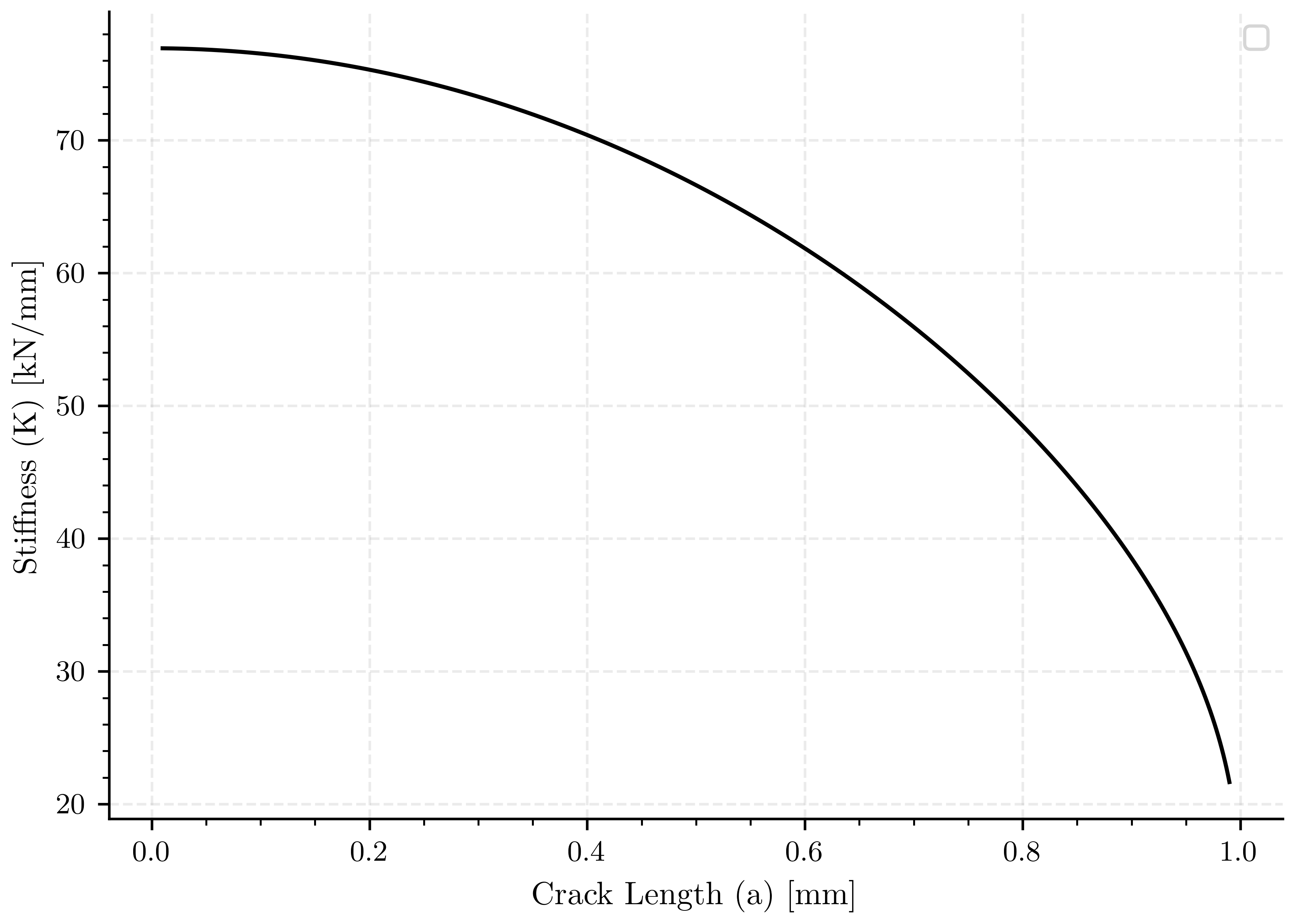
Compliance and stiffness calculations#
Compliance (C) and stiffness (K) are calculated using numerical integration. The compliance of the specimen witout crack is given by:
C0 = h / (Ep * b)  # Compliance of specimen without crack


# Define integration function using trapezoidal or Simpson's rule
from scipy.integrate import cumulative_trapezoid, cumulative_simpson

# Calculate compliance (C) and stiffness (K)
alpha = 2.0 # the crack propagates in both directions (2a)
C = C0/B * (1 + B / C0 * alpha*2.0 / (Ep * B * b) * cumulative_trapezoid(f_geometric**2, a, initial=0))  # Compliance
K = 1.0 / C  # Stiffness
Plot: Stiffness (\(K\)) vs. crack length (\(a\))#
fig, ax1 = plt.subplots()

ax1.plot(a, K, color=color_analytical, linestyle='-')  # Plot K vs. a

ax1.set_xlabel(pcfg.crack_length_label)  # Label for crack length
ax1.set_ylabel(pcfg.stiffness_label)  # Label for stiffness
ax1.legend()
/home/docs/checkouts/readthedocs.org/user_builds/phasefieldfatigue/checkouts/stable/examples/LEFM/plot_central_cracked.py:137: UserWarning: No artists with labels found to put in legend.  Note that artists whose label start with an underscore are ignored when legend() is called with no argument.
  ax1.legend()

<matplotlib.legend.Legend object at 0x734c65a49c30>
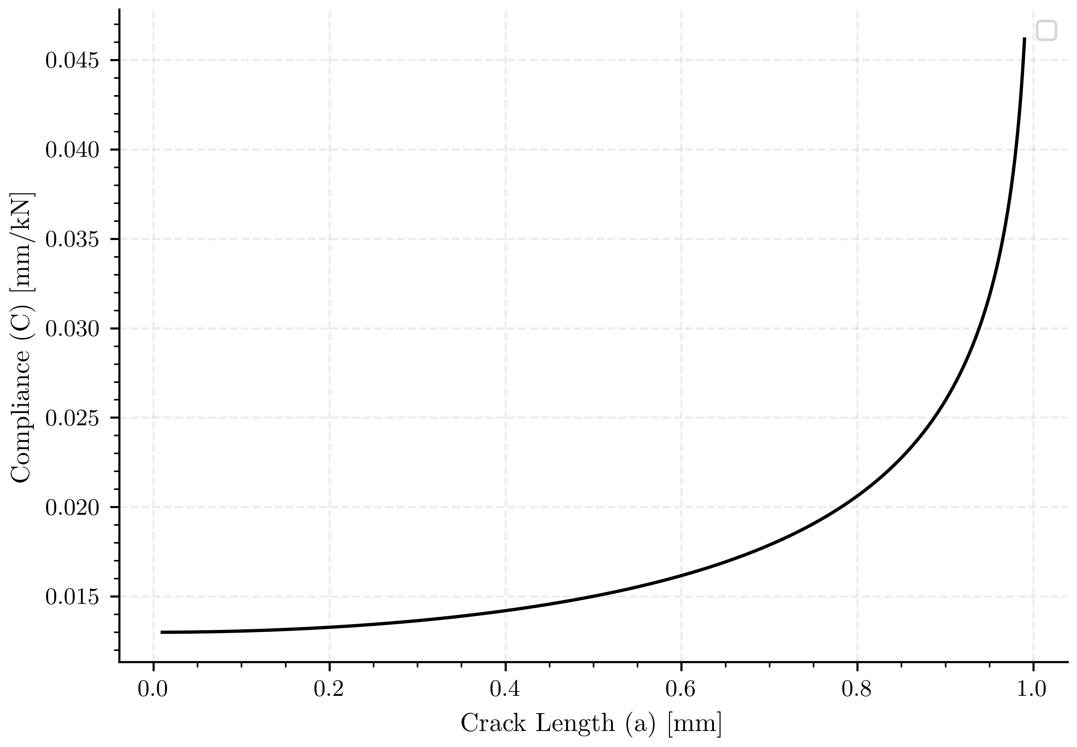
Plot: Compliance (\(C\)) vs. crack length (\(a\))#
fig, ax1 = plt.subplots()

ax1.plot(a, C, color=color_analytical, linestyle='-')

ax1.set_xlabel(pcfg.crack_length_label)
ax1.set_ylabel(pcfg.compliance_label)
ax1.legend()
/home/docs/checkouts/readthedocs.org/user_builds/phasefieldfatigue/checkouts/stable/examples/LEFM/plot_central_cracked.py:148: UserWarning: No artists with labels found to put in legend.  Note that artists whose label start with an underscore are ignored when legend() is called with no argument.
  ax1.legend()

<matplotlib.legend.Legend object at 0x734c658b03d0>
dC/da term#
This term is calculated as the derivative of compliance with respect to crack length note that the crack prpagates symetrically to the right and the left, so we use \(2a\) for the derivative.
dCda_numerical = np.gradient(C, 2*a)
Also is possible to obtain the relation directly by the following formula
dCda = 2*B*Gc / P_c**2

# Simple test to verify that the numerical and analytical dC/da are close
try:
    # Use a relative tolerance of 5% because numerical differentiation can
    # have inaccuracies.
    np.testing.assert_allclose(dCda_numerical, dCda, rtol=1e-2)
    print("Validation successful: Numerical dC/da matches analytical dC/da"
          " within tolerance.")
except AssertionError as e:
    print("Validation failed: Numerical and analytical dC/da do not match."
          f"\n{e}")


fig, ax1 = plt.subplots()
ax1.plot(a, dCda, color=color_analytical, linestyle='-', label='Analytical')  # Plot analytical dC/da
ax1.plot(a, dCda_numerical, color=color_quaternary, linestyle='--', label='Numerical')  # Plot numerical dC/da
ax1.grid(color='k', linestyle='-', linewidth=0.3)

ax1.set_xlabel(pcfg.crack_length_label)  # Label for crack length
ax1.set_ylabel(pcfg.dCda_label)
ax1.legend()
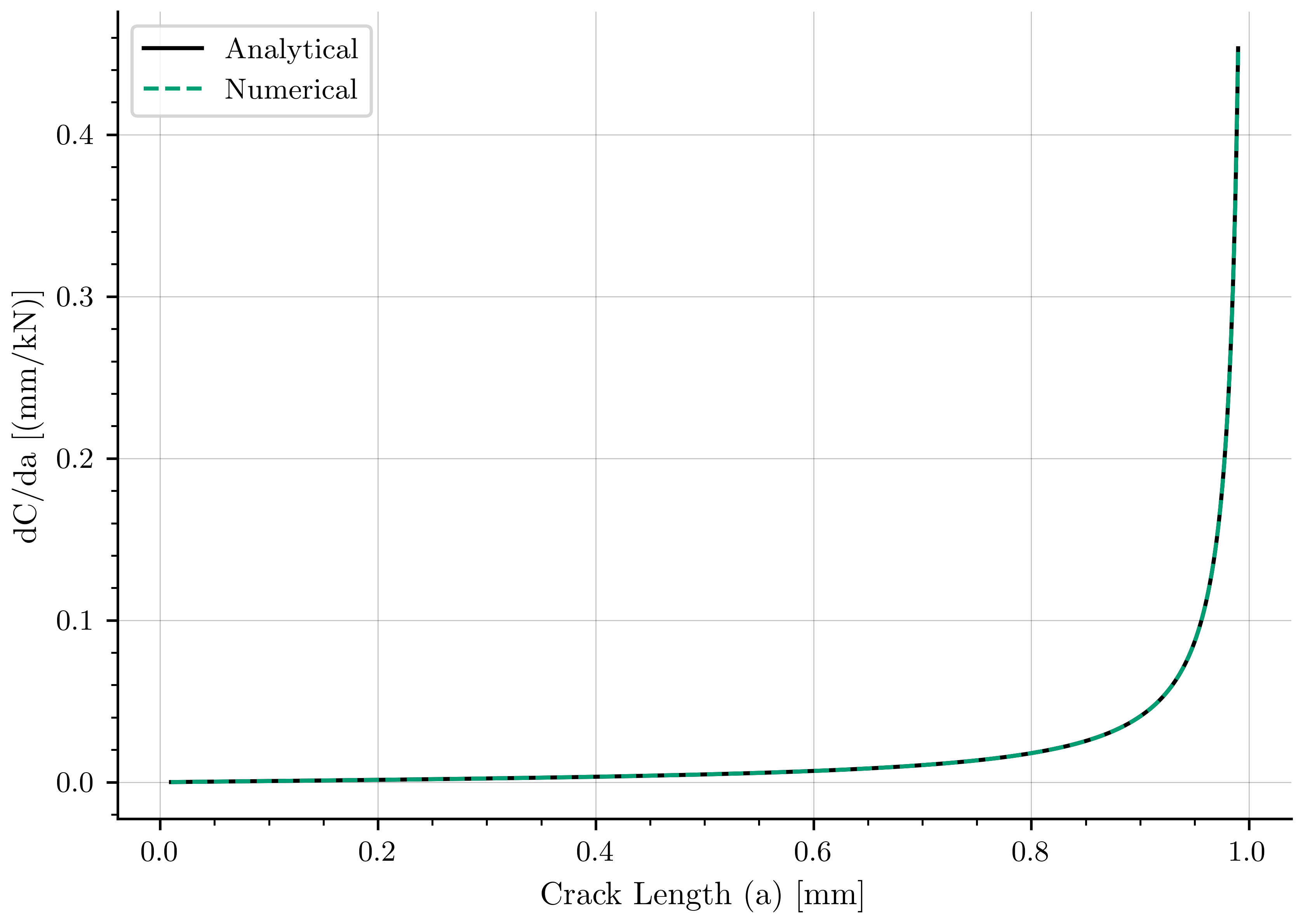
Validation successful: Numerical dC/da matches analytical dC/da within tolerance.

<matplotlib.legend.Legend object at 0x734c65809570>
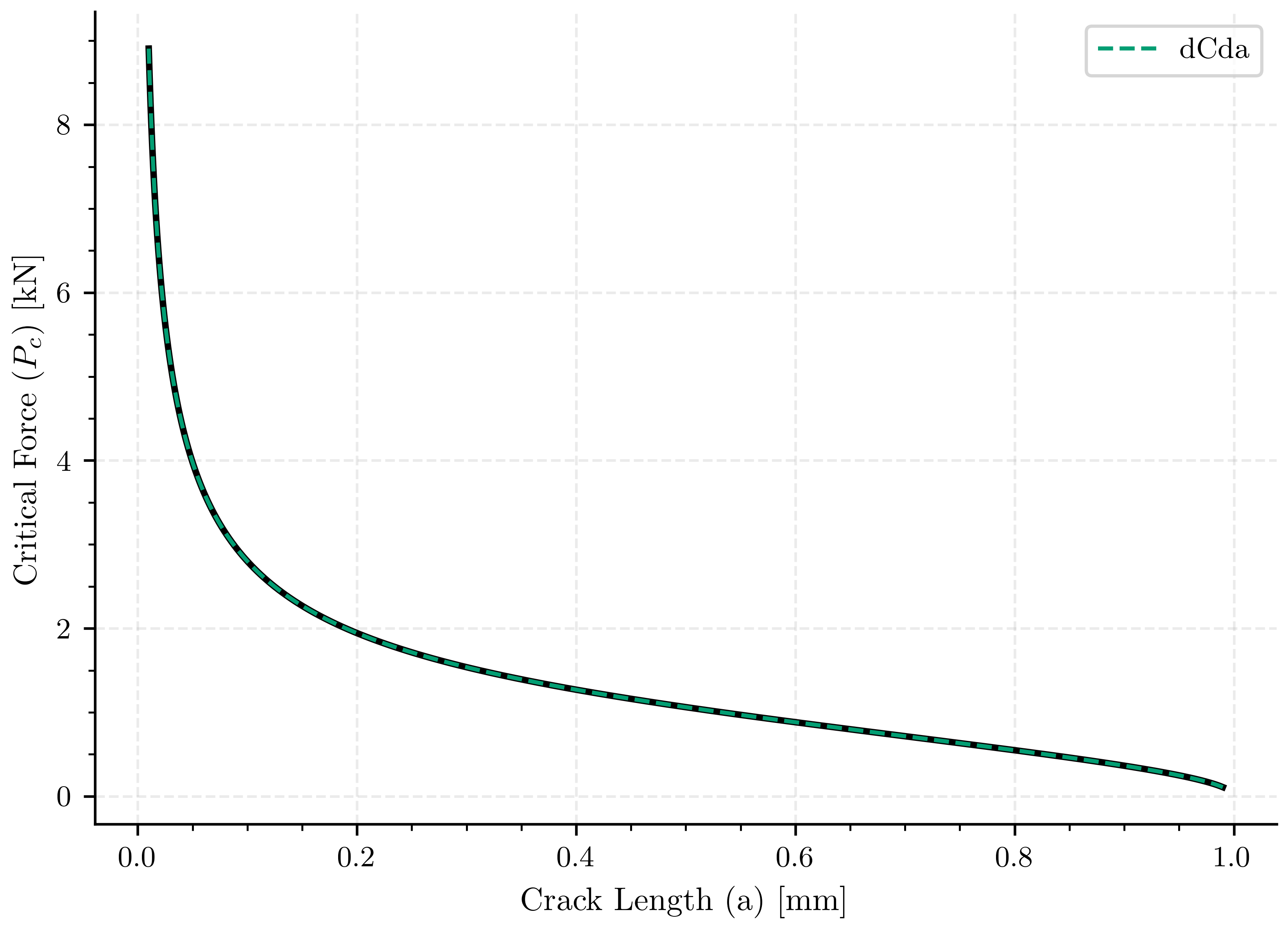
Plot: Critical force (\(P_c\)) vs. crack length (\(a\))#
fig, ax1 = plt.subplots()

ax1.plot(a, P_c, color=color_analytical, linestyle='-', linewidth=2.0)  # Plot P_c vs. a
ax1.plot(a, np.sqrt(2.0 *B* Gc / dCda), color=color_quaternary, linestyle='--', label='dCda')
ax1.set_xlabel(pcfg.crack_length_label)  # Label for crack length
ax1.set_ylabel(pcfg.critical_force_label)  # Label for critical force
ax1.legend()
<matplotlib.legend.Legend object at 0x734c63800790>
Save results to file#
results = np.column_stack((a, P_c, C, dCda))
header = "a\tPc\tC\tdCda"
np.savetxt(os.path.join(results_folder, "center_cracked.lefm"),
           results, fmt="%.6e", delimiter="\t", header=header, comments="")
Specific curves#
def get_u_P(ap0, a, P_c, C, Gc=Gc):
    index_ap0 = np.argmin(np.abs(a - ap0))
    P_c_a0 = P_c[index_ap0]
    u_c_a0 = P_c_a0 * C[index_ap0]

    u = P_c[index_ap0:] * C[index_ap0:]
    P = P_c[index_ap0:]
    a = a[index_ap0:]

    u0 = np.linspace(0, u[0], 1000)
    u = np.concatenate((u0, u))
    P = np.concatenate((u0 / C[index_ap0], P))
    a = np.concatenate((u0 * 0 + a[0], a))
    W = Gc * (a - ap0)
    C = u / P
    E = P**2 * C / 2
    # E = P*u / 2
    return u, P, a, W, E, u_c_a0, P_c_a0

# %
# Define specific crack length points for the analysis
ap0_points = np.array([0.3, 0.5, 0.7])  # Specific crack length points
ap0_colors = np.array(["red", "blue", "green"])  # Colors for these points in plots
ap0_style = ["-", "--", "--"]  # Line styles for these points
ap0_label = np.array([f"$a_0$={ap0_points[0]} mm", f"$a_0$={ap0_points[1]} mm ", f"$a_0$={ap0_points[2]} mm"])  # Labels for legend
index_ap0 = np.zeros(len(ap0_points), dtype=int)  # Indices of these points in the crack length array

# Find the indices of the specific crack length points in the array
i = 0
for a_i in ap0_points:
    index_ap0[i] = np.argmin(np.abs(a - a_i))  # Find the closest index
    i += 1

u1, P1, a1, W1, E1, u_c_a01, P_c_a01 = get_u_P(ap0_points[0], a, P_c, C)
u2, P2, a2, W2, E2, u_c_a02, P_c_a02 = get_u_P(ap0_points[1], a, P_c, C)
u3, P3, a3, W3, E3, u_c_a03, P_c_a03 = get_u_P(ap0_points[2], a, P_c, C)


header_curves = "a\tu\tP\tstrain_energy\tfracture_energy"
results_1 = np.column_stack((a1, u1, P1, E1, W1))
np.savetxt(
    os.path.join(
        results_folder,
        f"a0_{str(ap0_points[0]).replace('.', '')}.lefm_problem"
    ),
    results_1, fmt="%.6e", delimiter="\t", header=header_curves, comments=""
)

results_2 = np.column_stack((a2, u2, P2, E2, W2))
np.savetxt(
    os.path.join(
        results_folder,
        f"a0_{str(ap0_points[1]).replace('.', '')}.lefm_problem"
    ),
    results_2, fmt="%.6e", delimiter="\t", header=header_curves, comments=""
)

results_3 = np.column_stack((a3, u3, P3, E3, W3))
np.savetxt(
    os.path.join(
        results_folder,
        f"a0_{str(ap0_points[2]).replace('.', '')}.lefm_problem"
    ),
    results_3, fmt="%.6e", delimiter="\t", header=header_curves, comments=""
)

P_c_gc3 = B * np.sqrt(b) * np.sqrt(Ep * Gc*2) / f_geometric
P_c_gcdiv3 = B * np.sqrt(b) * np.sqrt(Ep * Gc / 2) / f_geometric
u2_gc3, P2_gc3, a2_gc3, W2_gc3, E2_gc3, u_c_a02_gc3, P_c_gc3 = get_u_P(ap0_points[1], a, P_c_gc3, C, Gc*2)
u2_gcdiv3, P2_gcdiv3, a2_gcdiv3, W2_gcdiv3, E2_gcdiv3, u_c_a02_gcdiv3, P_c_gcdiv3 = get_u_P(ap0_points[1], a, P_c_gcdiv3, C, Gc/2)
/home/docs/checkouts/readthedocs.org/user_builds/phasefieldfatigue/checkouts/stable/examples/LEFM/plot_central_cracked.py:222: RuntimeWarning: invalid value encountered in divide
  C = u / P
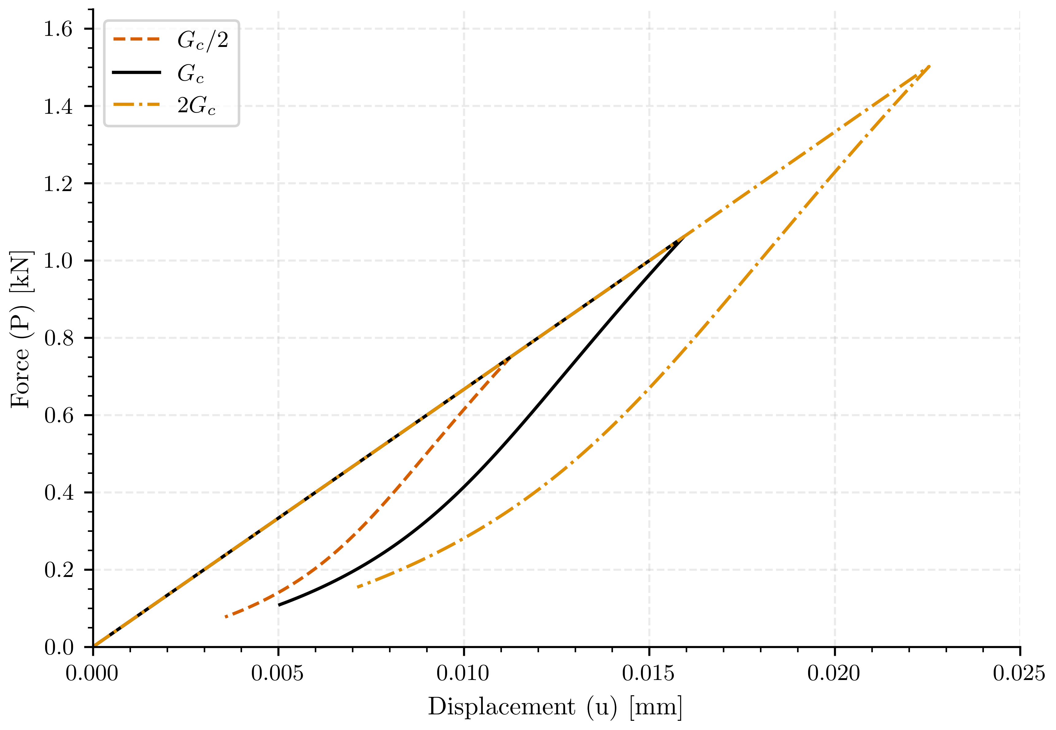
Plot: Displacement (\(u\)) vs. Force (\(P\))#
fig, ax1 = plt.subplots()

ax1.plot(u2_gcdiv3, P2_gcdiv3, color=color_secondary, linestyle='--', label=r"$G_c/2$")
ax1.plot(u2, P2, color=color_analytical, linestyle='-', label=r"$G_c$")
ax1.plot(u2_gc3, P2_gc3, color=color_tertiary, linestyle='-.', label=r"$2 G_c$")
ax1.set_xlim(0, 0.025)
ax1.set_ylim(0, 1.65)

ax1.set_xlabel(pcfg.displacement_label)
ax1.set_ylabel(pcfg.force_label)
ax1.legend()

# plt.savefig(os.path.join(results_folder, "compare_gc_force_vs_displacement"))
plt.show()
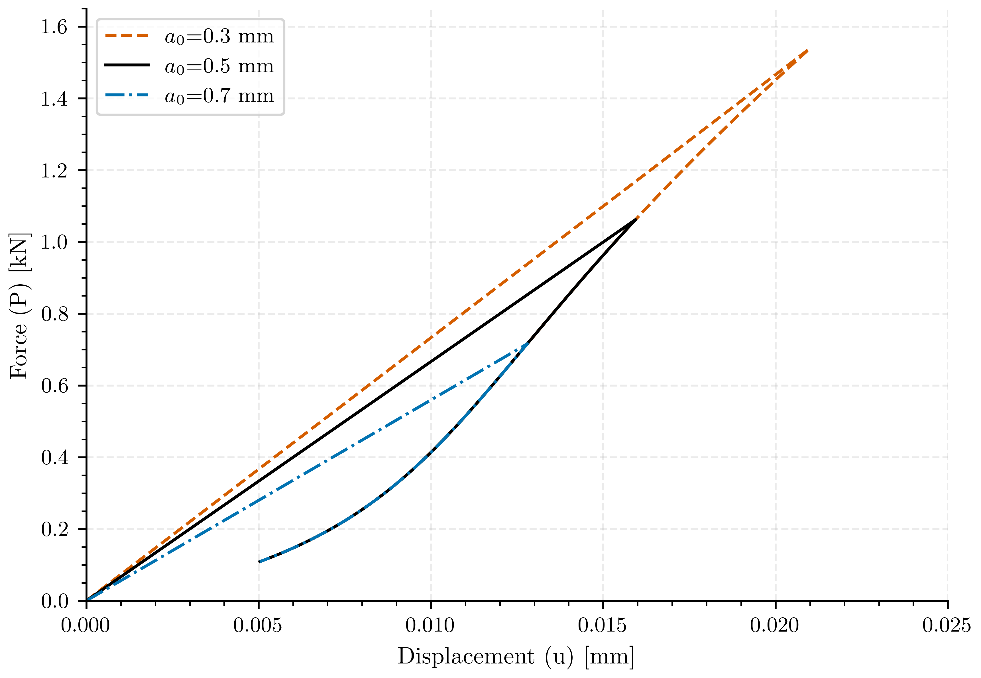
Plot: Displacement (\(u\)) vs. Force (\(P\))#
fig, ax1 = plt.subplots()

ax1.plot(u1, P1, color=color_secondary, linestyle='--', label=ap0_label[0])
ax1.plot(u2, P2, color=color_analytical, linestyle='-', label=ap0_label[1])
ax1.plot(u3, P3, color=color_main, linestyle='-.', label=ap0_label[2])

ax1.set_xlabel(pcfg.displacement_label)
ax1.set_ylabel(pcfg.force_label)
ax1.legend()
ax1.set_xlim(0, 0.025)
ax1.set_ylim(0, 1.65)
# plt.savefig(os.path.join(results_folder, "force_vs_displacement"))
plt.show()
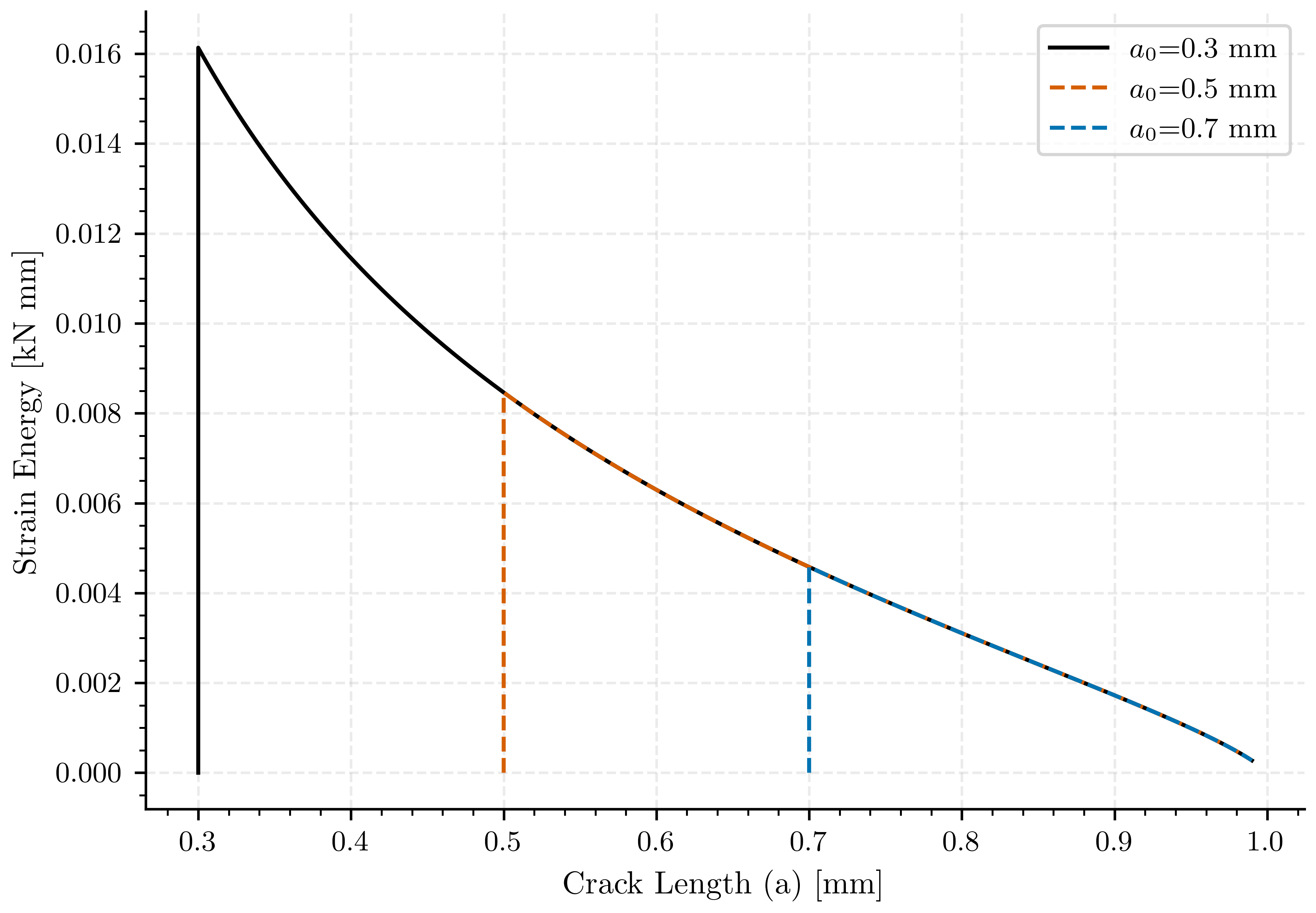
Plot: (\(a\)) vs. Energy (\(E\))#
fig, ax1 = plt.subplots()

ax1.plot(a1, E1, color=color_analytical, linestyle='-', label=ap0_label[0])
ax1.plot(a2, E2, color=color_secondary, linestyle='--', label=ap0_label[1])
ax1.plot(a3, E3, color=color_main, linestyle='--', label=ap0_label[2])

ax1.set_xlabel(pcfg.crack_length_label)
ax1.set_ylabel(pcfg.strain_energy_label)
ax1.legend()
<matplotlib.legend.Legend object at 0x734c63394640>
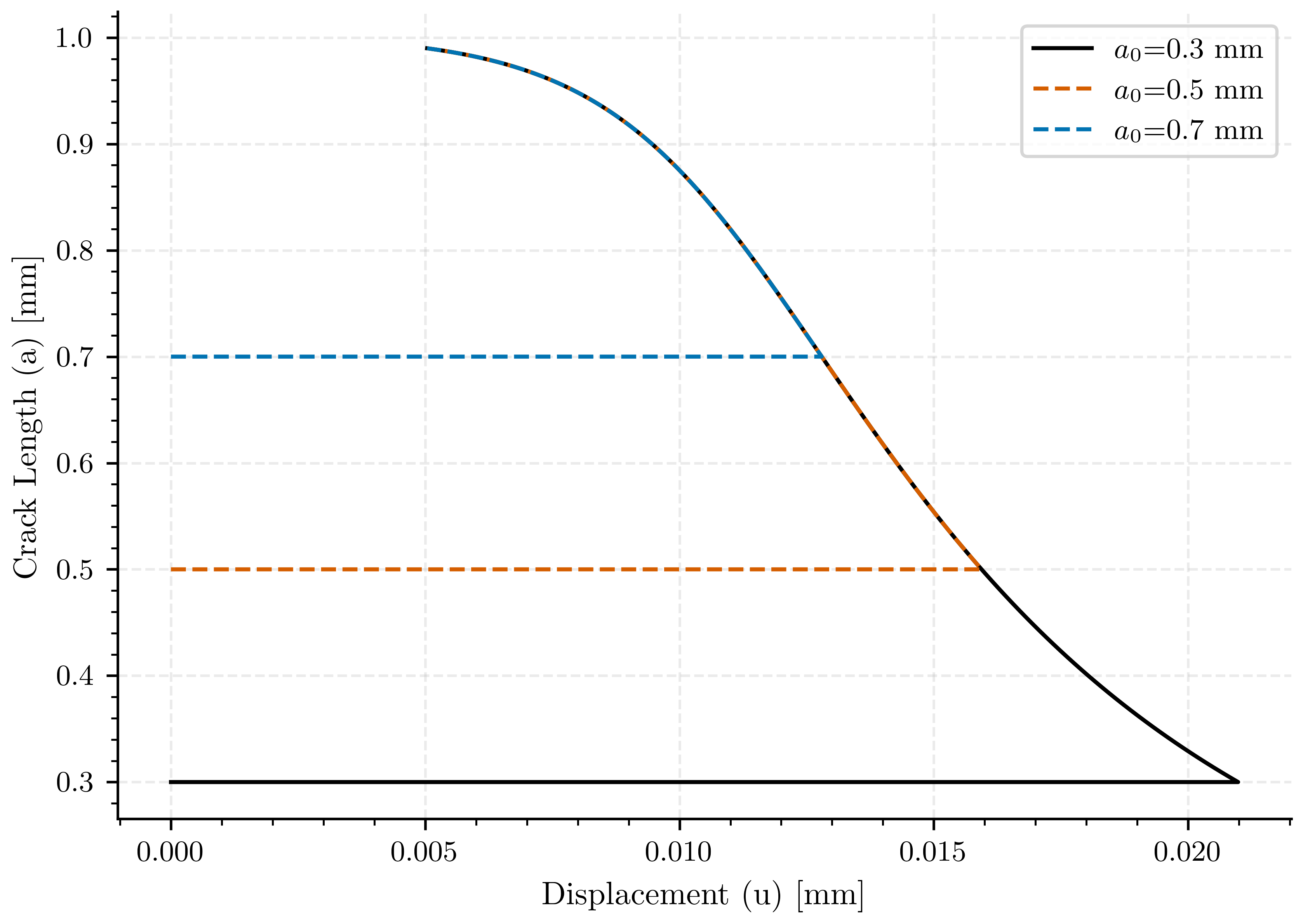
Energy calculations for a0=0.3 mm#
fig, ax1 = plt.subplots()

ax1.plot(u1, a1, color=color_analytical, linestyle='-', label=ap0_label[0])
ax1.plot(u2, a2, color=color_secondary, linestyle='--', label=ap0_label[1])
ax1.plot(u3, a3, color=color_main, linestyle='--', label=ap0_label[2])

ax1.set_xlabel(pcfg.displacement_label)
ax1.set_ylabel(pcfg.crack_length_label)
ax1.legend()
<matplotlib.legend.Legend object at 0x734c637683d0>
Fatigue Life Calculation and Validation#
a0_fatigue = 0.4 # Initial crack length [mm]
af_fatigue = 0.99 # Final crack length [mm]
To perform the fatigue analysis in that range, will be needed to tlice the arrays to obtain the values of the compliance and crack area in that range.
def slice_array_by_values(a, value_1, value_2):
    """
    Returns a slice of the array `a` between the indices of the nearest values to `value_1` and `value_2`.

    Parameters:
    a (numpy.ndarray): The input array.
    value_1 (float): The first value to find in the array.
    value_2 (float): The second value to find in the array.

    Returns:
    numpy.ndarray: A new array sliced between the indices of the nearest values to `value_1` and `value_2`.
    """
    # Find the indices of the nearest values
    index_1 = (np.abs(a - value_1)).argmin()
    index_2 = (np.abs(a - value_2)).argmin()

    # Ensure index_1 is less than index_2
    if index_1 > index_2:
        index_1, index_2 = index_2, index_1

    # Return the sliced array
    return index_1, index_2 + 1
Slice the arrays to obtain the fatigue region
i_o_1, i_f_1 = slice_array_by_values(a, a0_fatigue, af_fatigue)
a_fatigue = a[i_o_1:i_f_1]  # Crack lengths in the fatigue range
f_geometric_fatigue = f_geometric[i_o_1:i_f_1]
dCda_fatigue = dCda[i_o_1:i_f_1]  # Compliance derivative in the fatigue range

# This section calculates the fatigue life (number of cycles vs. crack length)
# using two theoretically equivalent LEFM approaches:
#
# 1. Stress-Based Method: Using the geometric factor f(a/W) to find Delta_K.
# 2. Energy-Based Method: Using the compliance derivative dC/da.
#
# The results are then compared to validate the numerical implementation.

# --- Fatigue Material Properties ---
AP = 33.0      # Applied cyclic force range (Delta_P) [kN]
Ni = 0         # Initial number of cycles

# --- Method 1: Fatigue Life from Geometric Factor ---
# Calculate the stress intensity factor range (Delta_K)
AK = AP / (B * np.sqrt(b)) * f_geometric_fatigue  # Stress intensity factor range
# Integrate Paris' Law: Nf = integral(1 / (C * (Delta_K)^m)) da
# For numerical stability, constant terms are pulled out of the integral.
Nf_f_geometric = Ni + 1/(Cparis * (AP/(B*np.sqrt(b)))**m) * \
    cumulative_trapezoid(1/(f_geometric_fatigue**m), a_fatigue, initial=0)
# Nf_f_geometric = Ni + cumulative_trapezoid(1 / (Cparis * AK**m), a, initial=0)

# --- Method 2: Fatigue Life from Compliance Derivative (dC/da) ---
# This uses the energy-based formulation of Paris' Law.
Nf_dCda = Ni + 1 / (Cparis * (Ep / (2 * B))**(m / 2) * AP**m) * \
    cumulative_trapezoid(1 / (dCda_fatigue)**(m / 2), a_fatigue, initial=0)

# --- Validation Test ---
# Verify that both methods produce nearly identical results. A small tolerance
# is required to account for numerical errors from integration and differentiation.
try:
    # Use a relative tolerance of 1% (rtol=1e-2).
    np.testing.assert_allclose(Nf_f_geometric, Nf_dCda, rtol=1e-2)
    print("Validation successful: Fatigue life calculations from geometric"
          " factor and dC/da are consistent.")
except AssertionError as e:
    print("Validation FAILED: The two fatigue life calculation methods do not"
          f" match.\n{e}")
Validation successful: Fatigue life calculations from geometric factor and dC/da are consistent.
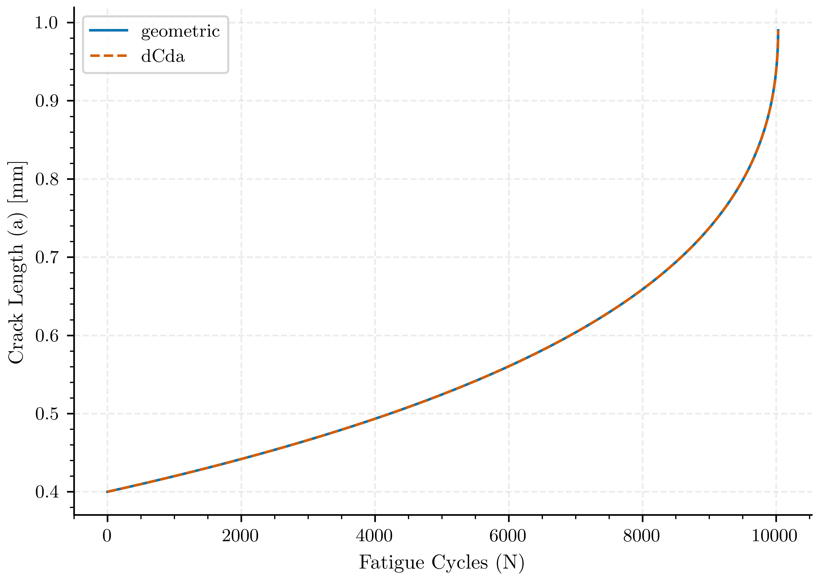
Plot:#
fig, ax1 = plt.subplots()

ax1.plot(Nf_f_geometric, a_fatigue, color=color_main, linestyle='-', label=r"geometric")
ax1.plot(Nf_dCda, a_fatigue, color=color_secondary, linestyle='--', label=r"dCda")

ax1.set_xlabel(pcfg.cycles_label)
ax1.set_ylabel(pcfg.crack_length_label)
ax1.legend()

plt.show()

header_fatigue = "cycles\ta"
results_fatigue = np.column_stack((Nf_dCda, a_fatigue))
np.savetxt(
    os.path.join(
        results_folder,
        f"a_{str(a0_fatigue).replace('.', '')}_{str(af_fatigue).replace('.', '')}.lefm_fatigue"
    ),
    results_fatigue, fmt="%.6e", delimiter="\t", header=header_fatigue, comments=""
)
Total running time of the script: (0 minutes 16.603 seconds)