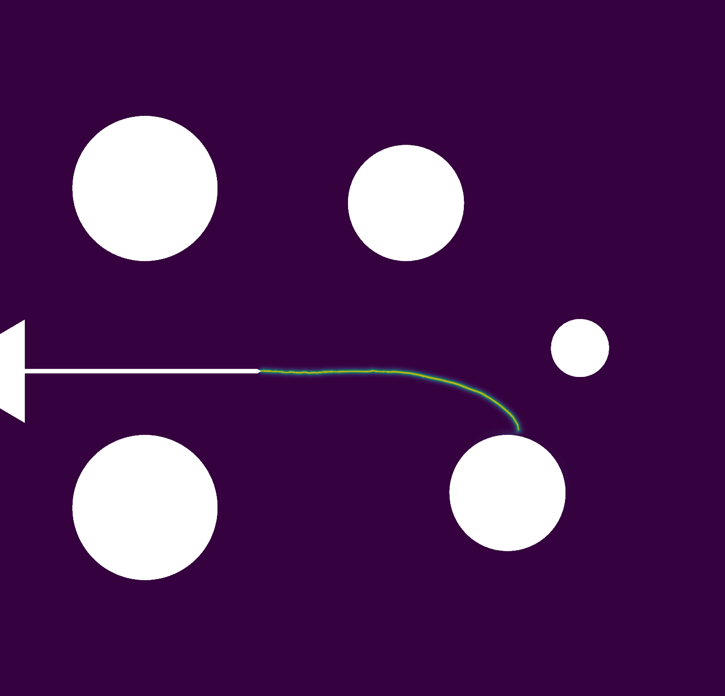
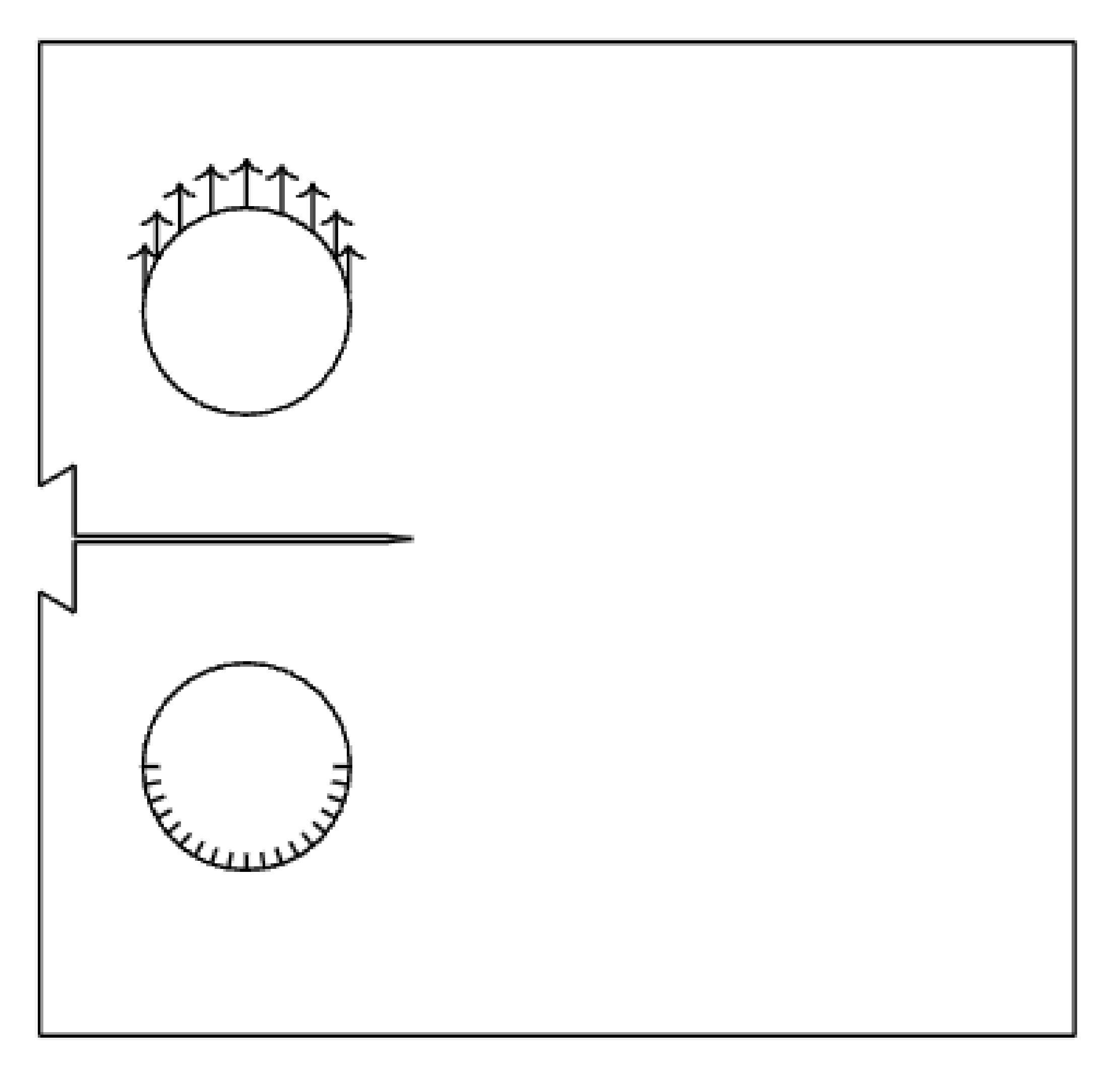
Comparison: Specimen 1

This script generates a plot comparing the stiffness the compact specimen as a function of crack length. The results include four different approaches:

• Phase-field simulation: Stiffness values obtained under displacement-controlled conditions. The phase-field simulation results are generated in the script ref_phase_field_compact_specimen_0_H00.

• Force-Controlled Loading: Stiffness values obtained under force-controlled conditions. The force-controlled simulation results are generated in the script Force Controlled Compact Specimen.

• LEFM Theory: Theoretical predictions based on Linear Elastic Fracture Mechanics (LEFM). The LEFM results are generated in the script Compact Tension Specimen: Fracture and Fatigue Analysis.

Finally, the script also includes results from a phase-field simulation of a centrally cracked specimen.

The purpose of this script is to visualize and compare the stiffness behavior of the specimen under different loading conditions and theoretical predictions.

Import necessary libraries

import numpy as np
from scipy.integrate import cumulative_trapezoid
import matplotlib.pyplot as plt
import pandas as pd
import matplotlib.image as mpimg
import os
import sys

sys.path.insert(0, os.path.abspath('../../'))
plt.style.use('../../graph.mplstyle')
import plot_config as pcfg

img = mpimg.imread('images/compact_specimen.png')
plt.imshow(img)
plt.axis('off')

results_folder = "compact_tension"
os.makedirs(results_folder, exist_ok=True)

Parameters definition

Define material and specimen parameters

E   = 211     # Young's modulus (kN/mm^2)
nu  = 0.3     # Poisson's ratio (-)
Gc  = 0.073   # Critical strain energy release rate (kN/mm)
Ep = E / (1.0 - nu**2) # Plane strain modulus (kN/mm^2)

Define specimen geometry

a0 = 8.0
W  = 40.0  # Characteristic width of the specimen (mm)
B  = 3.2   # Thickness (mm)

m = 2.08     # Paris' Law exponent (-)
Cparis = 1.615*10**(-8) * 10**(3*m/2)

Ni = 0   # [cycles] Initial number of cycles
R = 0.1  # [-] Load ratio

theta = 0.04 # mm^-1
K0 = 15.0 * 1/(10*np.sqrt(10))
G0 = K0**2/(Ep)

Load the results

From Linear elastic fracture mechanics theory LEFM: Center-Cracked Specimen

label_lefm = r"LEFM"
color_lefm = pcfg.color_black
SCHEME_1 = np.loadtxt("../LEFM/results_compact_specimen/results.lefm", delimiter="\t", skiprows=1)
a_lefm = SCHEME_1[:,0]
k_lefm = SCHEME_1[:,1]
c_lefm = 1/k_lefm
dCda_lefm = np.gradient(c_lefm, a_lefm)

From FEM elastic force controlled simulation Force Controlled Center Cracked Specimen

label_force = r"Elasticity"
color_force = pcfg.color_orangered
results_elasticity = pd.read_csv("../Elasticity/results_compact_tension_gmsh/results.elasticity", delimiter="\t", comment="#", header=0)
a_forc = results_elasticity["a"]
k_forc = results_elasticity["stiffness"]*B
c_forc = results_elasticity["compliance"]/B
dCda_forc = np.gradient(c_forc, a_forc)

From phase-field fracture with Bourdin correction

label_pff_bourdin = r"Phase-Field: Bourdin"
color_pff_bourdin = pcfg.color_purple
results_pff_bourdin = pd.read_csv("../Phase_Field_Compact_Specimen/results_specimen_1_H00/results_corrected_bourdin.pff", delimiter="\t", comment="#", header=0)

k_pff_bourdin = 1/results_pff_bourdin["compliance"] * B
c_pff_bourdin = results_pff_bourdin["compliance"] / B

a_pff_bourdin = results_pff_bourdin["gamma"]
dCda_pff_bourdin = results_pff_bourdin["dCda"]/B

force_pff_bourdin = results_pff_bourdin["force"] *B
u_pff_bourdin = results_pff_bourdin["displacement"]

From phase-field fracture with skeleton correction

label_pff_geo = r"Phase-Field: Skeleton"
color_pff_geo = pcfg.color_blue
results_pff_geo = pd.read_csv("../Phase_Field_Compact_Specimen/results_specimen_1_H00/results_corrected_geometry.pff", delimiter="\t", comment="#", header=0)

k_pff_geo = 1/results_pff_geo["compliance"] * B
c_pff_geo = results_pff_geo["compliance"] / B

a_pff_geo = results_pff_geo["gamma"]
dCda_pff_geo = results_pff_geo["dCda"]/B

force_pff_geo = results_pff_geo["force"] *B
u_pff_geo = results_pff_geo["displacement"]


markevery_pff_bourdin = max(1, len(a_pff_bourdin)//10)
markevery_pff_geo = max(1, len(a_pff_geo)//10)
markevery_forc = max(1, len(a_forc)//10)
markevery_lefm = max(1, len(a_lefm)//10)

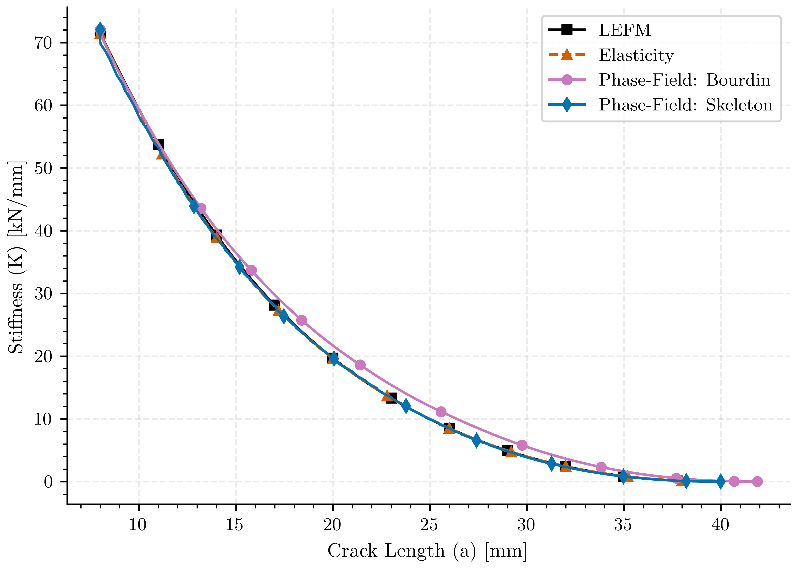
Crack length vs stiffness

The stiffness as function of crack length is plotted for the three methods.

fig, ax0 = plt.subplots()

ax0.plot(a_lefm, k_lefm, color=color_lefm, linestyle='-', marker='s', markevery=markevery_lefm, label=label_lefm)
ax0.plot(a_forc, k_forc, color=color_force, linestyle='--', marker='^', markevery=markevery_forc, label=label_force)
ax0.plot(a_pff_bourdin,  k_pff_bourdin, color=color_pff_bourdin, linestyle='-', marker='o', markevery=markevery_pff_bourdin, label=label_pff_bourdin)
ax0.plot(a_pff_geo,  k_pff_geo, color=color_pff_geo, linestyle='-', marker='d', markevery=markevery_pff_geo, label=label_pff_geo)

ax0.set_xlabel(pcfg.crack_length_label)
ax0.set_ylabel(pcfg.stiffness_label)
ax0.legend()
plt.savefig(os.path.join(results_folder, "compare_stiffness"))

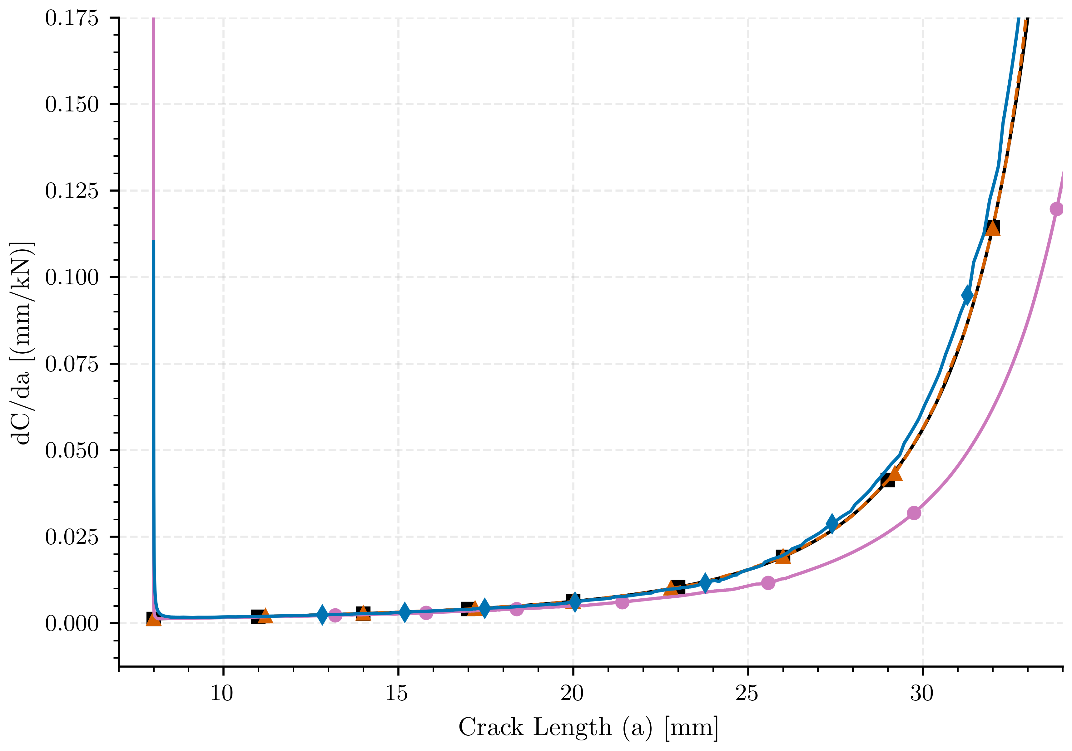
Crack area vs \(dC/da\)

The derivative of the compliance respect the crack area is plotted for the three methods.

fig, ax2 = plt.subplots()

ax2.plot(a_lefm, dCda_lefm, color=color_lefm, linestyle='-', marker='s', markevery=markevery_lefm, label=label_lefm)
ax2.plot(a_forc, dCda_forc, color=color_force, linestyle='--', marker='^', markevery=markevery_forc, label=label_force)
ax2.plot(a_pff_bourdin,  dCda_pff_bourdin, color=color_pff_bourdin, linestyle='-', marker='o', markevery=markevery_pff_bourdin, label=label_pff_bourdin)
ax2.plot(a_pff_geo,  dCda_pff_geo, color=color_pff_geo, linestyle='-', marker='d', markevery=markevery_pff_geo, label=label_pff_geo)

ax2.set_xlabel(pcfg.crack_length_label)
ax2.set_ylabel(pcfg.dCda_label)
ax2.set_ylim(bottom=-0.0125, top=0.175)  # Set the top y-limit
ax2.set_xlim(left=7.0, right=34.0)  # Set the top y-limit

# ax2.legend()
plt.savefig(os.path.join(results_folder, "dCda_vs_crack_length"))

Fatigue

Once the compliance curves are obtained, it is possible to calculate the fatigue lives from the compliance respect the crack area for the different methods. In this case the fatigue analysis is performed for a crack that goes from an initial crack length value_1 to a final crack length value_2.

pre_crack = 3.5
a0_fatigue = 0.2*W + pre_crack # Initial crack length [mm]
af_fatigue = 0.99*W # Final crack length [mm]

To perform the fatigue analysis in that range, will be needed to tlice the arrays to obtain the values of the compliance and crack area in that range.

def slice_array_by_values(a, value_1, value_2):
    """
    Returns a slice of the array `a` between the indices of the nearest values to `value_1` and `value_2`.

    Parameters:
    a (numpy.ndarray): The input array.
    value_1 (float): The first value to find in the array.
    value_2 (float): The second value to find in the array.

    Returns:
    numpy.ndarray: A new array sliced between the indices of the nearest values to `value_1` and `value_2`.
    """
    # Find the indices of the nearest values
    index_1 = (np.abs(a - value_1)).argmin()
    index_2 = (np.abs(a - value_2)).argmin()

    # Ensure index_1 is less than index_2
    if index_1 > index_2:
        index_1, index_2 = index_2, index_1

    # Return the sliced array
    return index_1, index_2 + 1

Slice the arrays to obtain the fatigue region

i_o_2, i_f_2 = slice_array_by_values(a_forc, a0_fatigue, af_fatigue)
i_o_3, i_f_3 = slice_array_by_values(a_lefm, a0_fatigue, af_fatigue)
i_o_4, i_f_4 = slice_array_by_values(a_pff_bourdin,  a0_fatigue, af_fatigue)
i_o_5, i_f_5 = slice_array_by_values(a_pff_geo, a0_fatigue, af_fatigue)

i_f_4 = -1
i_f_5 = -1

Extract the fatigue regions

a_fatigue_forc, c_fatigue_forc = np.array(a_forc[i_o_2:i_f_2]), np.array(c_forc[i_o_2:i_f_2])
a_fatigue_lefm, c_fatigue_lefm = np.array(a_lefm[i_o_3:i_f_3]), np.array(c_lefm[i_o_3:i_f_3])
a_fatigue_pff,  c_fatigue_pff  = np.array(a_pff_bourdin[i_o_4:i_f_4]), np.array(c_pff_bourdin[i_o_4:i_f_4])
a_fatigue_pff_geo, c_fatigue_pff_geo  = np.array(a_pff_geo[i_o_5:i_f_5]), np.array(c_pff_geo[i_o_5:i_f_5])

Then, the derivative of the compliance respect the crack area is calculated for each method.

dCda_fatigue_forc = dCda_forc[i_o_2:i_f_2]
dCda_fatigue_lefm = dCda_lefm[i_o_3:i_f_3]
dCda_fatigue_pff = dCda_pff_bourdin[i_o_4:i_f_4]
dCda_fatigue_pff_geo = dCda_pff_geo[i_o_5:i_f_5]

P_fatigue_lefm = np.sqrt(2*B*G0 / dCda_lefm[i_o_3])   # Applied cyclic force range (Delta_P) [kN]
P_fatigue_forc = np.sqrt(2*B*G0 / dCda_forc[i_o_2])
P_fatigue_pff  = np.sqrt(2*B*G0 / dCda_pff_bourdin[i_o_4])
P_fatigue_pff_geo = np.sqrt(2*B*G0 / dCda_pff_geo[i_o_5])

Once, the derivative of the compliance respect the crack area is calculated, it is possible to calculate the number of cycles to failure using the Paris law. In this case, the Paris law is used in the form:

\[N_f = N_i + \frac{1}{C (E'/2B)^{n/2} ((1-R) P_\text{max})^{n}} \int_{a_i}^{a_f} \frac{\mathrm{d}a}{(\mathrm{d}C/\mathrm{d}a)^{n/2} \ e^{n \theta(a-a_i)}}.\]

Nf_dCda_elasticity = Ni + 1/(Cparis * (Ep/(2*B))**(m/2) * ((1-R)*P_fatigue_forc)**m)*cumulative_trapezoid(1/(dCda_fatigue_forc)**(m/2) * 1/(np.exp(m*theta*(a_fatigue_forc-a_fatigue_forc[0]))), x=a_fatigue_forc, initial=0)
Nf_dCda_lefm       = Ni + 1/(Cparis * (Ep/(2*B))**(m/2) * ((1-R)*P_fatigue_lefm)**m)*cumulative_trapezoid(1/(dCda_fatigue_lefm)**(m/2) * 1/(np.exp(m*theta*(a_fatigue_lefm-a_fatigue_lefm[0]))), x=a_fatigue_lefm, initial=0)
Nf_dCda_pff_bourdin= Ni + 1/(Cparis * (Ep/(2*B))**(m/2) * ((1-R)*P_fatigue_pff)**m)*cumulative_trapezoid(1/(dCda_fatigue_pff)**(m/2) * 1/(np.exp(m*theta*(a_fatigue_pff-a_fatigue_pff[0]))),  x=a_fatigue_pff,  initial=0)
Nf_dCda_pff_geo    = Ni + 1/(Cparis * (Ep/(2*B))**(m/2) * ((1-R)*P_fatigue_pff_geo)**m)*cumulative_trapezoid(1/(dCda_fatigue_pff_geo)**(m/2) * 1/(np.exp(m*theta*(a_fatigue_pff_geo-a_fatigue_pff_geo[0]))),  x=a_fatigue_pff_geo,  initial=0)

Crack length vs number of cycles

The number of cycles to failure is calculated from the compliance respect the crack area for the different methods.

fig, ax3 = plt.subplots(figsize=(11.69, 5.85))

ax3.plot(Nf_dCda_lefm, a_fatigue_lefm, color=color_lefm, linestyle='-', marker='s', markevery=markevery_lefm, label=label_lefm)
ax3.plot(Nf_dCda_elasticity, a_fatigue_forc, color=color_force, linestyle='--', marker='^', markevery=markevery_forc, label=label_force)
ax3.plot(Nf_dCda_pff_bourdin, a_fatigue_pff, color=color_pff_bourdin, linestyle='-', marker='o', markevery=markevery_pff_bourdin, label=label_pff_bourdin)
ax3.plot(Nf_dCda_pff_geo, a_fatigue_pff_geo, color=color_pff_geo, linestyle='-', marker='d', markevery=markevery_pff_geo, label=label_pff_geo)
# Enhance plot aesthetics
ax3.set_ylabel(pcfg.crack_length_label)
ax3.set_xlabel(pcfg.cycles_label)
ax3.legend()
plt.savefig(os.path.join(results_folder, "cycles_vs_crack_length"))

plt.show()


# Calculate percentage difference for each simulation vs experiment
percent_diff_elasticity = 100 * abs(Nf_dCda_elasticity[-1] - Nf_dCda_lefm[-1]) / Nf_dCda_lefm[-1]
percent_diff_pff = 100 * abs(Nf_dCda_pff_bourdin[-1] - Nf_dCda_lefm[-1]) / Nf_dCda_lefm[-1]
percent_diff_pff_geo = 100 * abs(Nf_dCda_pff_geo[-1] - Nf_dCda_lefm[-1]) / Nf_dCda_lefm[-1]

print(f"Percentage difference elasticity: {percent_diff_elasticity:.2f}%")
print(f"Percentage difference bourdin: {percent_diff_pff:.2f}%")
print(f"Percentage difference geo: {percent_diff_pff_geo:.2f}%")

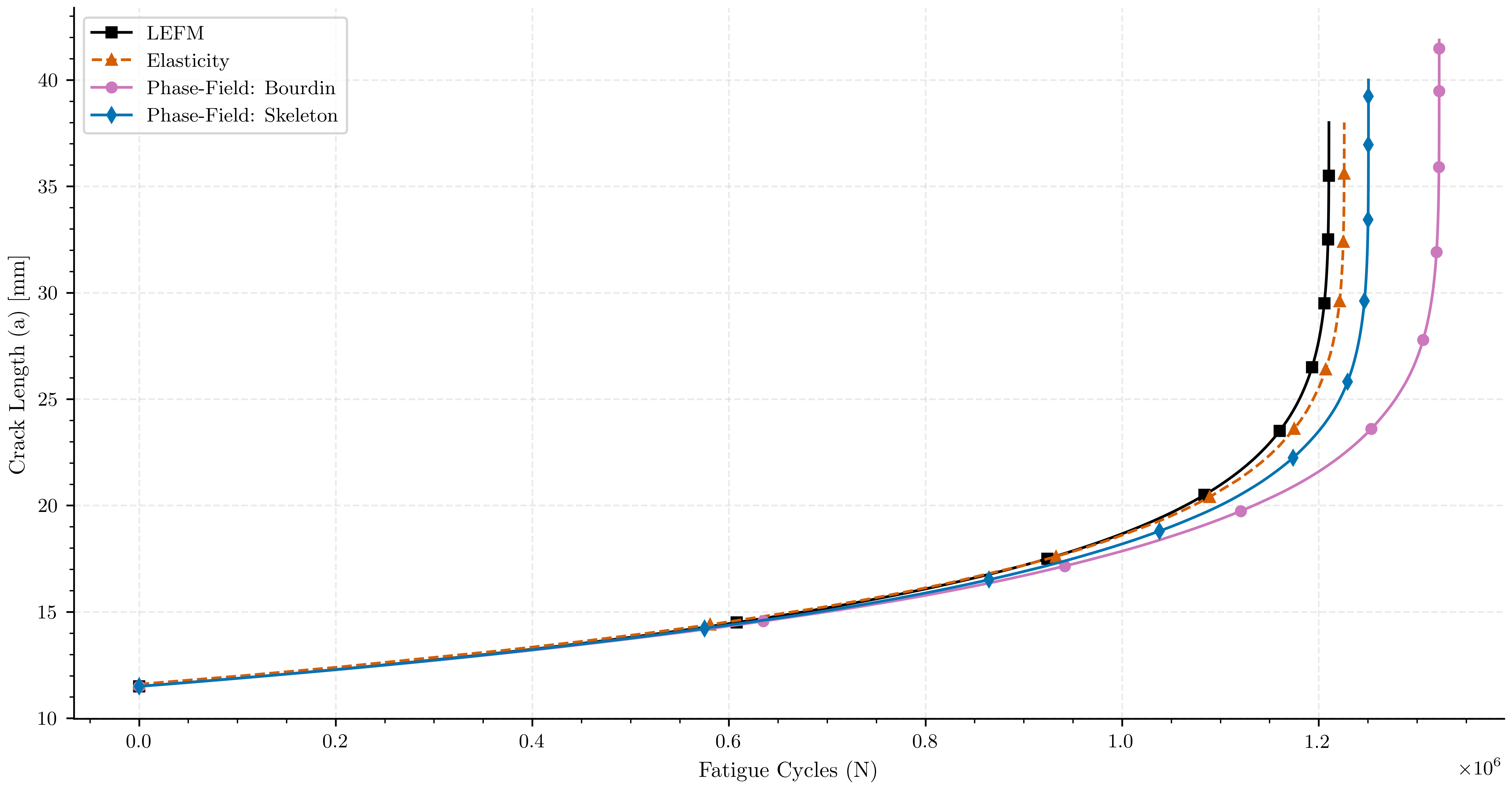
Percentage difference elasticity: 1.29%
Percentage difference bourdin: 9.27%
Percentage difference geo: 3.32%