Note
Go to the end to download the full example code.
Simulation 3#
The model represents a square plate with a central crack, as shown in the figure below. The bottom part is fixed in all directions, while the upper part can slide vertically. A vertical displacement is applied at the top. The geometry and boundary conditions are depicted in the figure. We discretize the model with quadrilateral elements.
Note
In this case, only one quarter of the model will be considered due to symmetry. Additionally, a regular mesh will be used.
#           u/\/\/\/\/\/\       u/\/\/\/\/\/\
#            ||||||||||||        ||||||||||||
#            *----------*    o|\ *----------*
#            |          |    o|/ |          |
#            | 2a=1.0   |    o|\ | a=a0     |
#            |   ----   |    o|/ *----------*
#            |          |             /_\/_\
#            |          |            oo oo oo
#            *----------*
#            /_\/_\/_\/_\
#     |Y    /////////////
#     |
#     *---X
The Young’s modulus, Poisson’s ratio, and the critical energy release rate are given in the table Properties. Young’s modulus \(E\) and Poisson’s ratio \(\nu\) can be represented with the Lamé parameters as: \(\lambda=\frac{E\nu}{(1+\nu)(1-2\nu)}\); \(\mu=\frac{E}{2(1+\nu)}\).
VALUE |
UNITS |
|
|---|---|---|
E |
210 |
kN/mm2 |
nu |
0.3 |
[-] |
Gc |
0.0027 |
kN/mm |
l |
0.015 |
mm |
Import necessary libraries#
import numpy as np
import dolfinx
import mpi4py
import petsc4py
import os
Import from phasefieldx package#
from phasefieldx.Element.Phase_Field_Fracture.Input import Input
from phasefieldx.Element.Phase_Field_Fracture.solver.solver_ener_non_variational import solve
from phasefieldx.Boundary.boundary_conditions import bc_y, bc_x, get_ds_bound_from_marker
from phasefieldx.PostProcessing.ReferenceResult import AllResults
Parameters Definition#
Data is an input object containing essential parameters for simulation setup and result storage:
E: Young’s modulus, set to 210 \(kN/mm^2\).
nu: Poisson’s ratio, set to 0.3.
Gc: Critical energy release rate, set to 0.0027 \(kN/mm\).
l: Length scale parameter, set to 0.025 \(mm\).
degradation: Specifies the degradation type. Options are “isotropic” or “anisotropic”.
split_energy: Controls how the energy is split; options include “no” (default), “spectral,” or “deviatoric.”
degradation_function: Specifies the degradation function; here, it is “quadratic.”
irreversibility: Not used/implemented for this solver.
save_solution_xdmf and save_solution_vtu: Specify the file formats to save displacement results. In this case, results are saved as .vtu files.
results_folder_name: Name of the folder for saving results. If it exists, it will be replaced with a new empty folder.
Data = Input(E=210.0,
             nu=0.3,
             Gc=0.0027,
             l=0.025,
             degradation="isotropic",
             split_energy="not_applied",
             degradation_function="quadratic",
             irreversibility="not_applied",
             fatigue=False,
             fatigue_degradation_function="not_applied",
             fatigue_val=None,
             k=0.0,
             save_solution_xdmf=False,
             save_solution_vtu=True,
             results_folder_name="results_3_a05_l1")
Mesh Definition#
The mesh is a structured grid with quadrilateral elements:
divx, divy: Number of elements along the x and y axes.
lx, ly: Physical domain dimensions in x and y.
divx, divy = 100, 300
lx, ly = 1.0, 3.0
h = ly / divy
msh = dolfinx.mesh.create_rectangle(mpi4py.MPI.COMM_WORLD,
                                    [np.array([0.0, 0.0]),
                                     np.array([lx, ly])],
                                    [divx, divy],
                                    cell_type=dolfinx.mesh.CellType.quadrilateral)

fdim = msh.topology.dim - 1 # Dimension of the mesh facets
The variable a0 defines the initial crack length in the mesh. This parameter is crucial for setting up the simulation, as it determines the starting point of the crack in the domain.
a0 = 0.5 # Initial crack length in the mesh
Boundary Identification Functions#
These functions identify points on the specific boundaries of the domain where boundary conditions will be applied. The bottom function checks if a point lies on the bottom boundary, returning True for points where y=0 and x is greater than or equal to a0. The top function identifies points on the top boundary, returning True for points where y=ly. The left function identifies points on the left boundary, returning True for points where x=0. and x is greater than or equal to -surface, and False otherwise.
This approach ensures that boundary conditions are applied to specific parts of the mesh, which helps in defining the simulation’s physical constraints.
def bottom(x):
    return np.logical_and(np.isclose(x[1], 0), np.greater_equal(x[0], a0))

def top(x):
    return np.isclose(x[1], ly)

def left(x):
    return np.isclose(x[0], 0.0)
Using the bottom, top, and left functions, we locate the facets on the respective boundaries of the mesh: - bottom: Identifies facets on the bottom boundary where y = 0 and x >= a0. - top: Identifies facets on the top boundary where y = ly. - left: Identifies facets on the left boundary where x = 0. The locate_entities_boundary function returns an array of facet indices representing these identified boundary entities.
bottom_facet_marker = dolfinx.mesh.locate_entities_boundary(msh, fdim, bottom)
top_facet_marker = dolfinx.mesh.locate_entities_boundary(msh, fdim, top)
left_facet_marker = dolfinx.mesh.locate_entities_boundary(msh, fdim, left)
The get_ds_bound_from_marker function generates a measure for applying boundary conditions specifically to the surface marker where the load will be applied, identified by top_facet_marker. This measure is then assigned to ds_top.
ds_top = get_ds_bound_from_marker(top_facet_marker, msh, fdim)
ds_list is an array that stores boundary condition measures along with names for each boundary, simplifying result-saving processes. Each entry in ds_list is formatted as [ds_, “name”], where ds_ represents the boundary condition measure, and “name” is a label used for saving. Here, ds_bottom and ds_top are labeled as “bottom” and “top”, respectively, to ensure clarity when saving results.
ds_list = np.array([
                   [ds_top, "top"],
                   ])
Function Space Definition#
Define function spaces for displacement and phase-field using Lagrange elements.
V_u = dolfinx.fem.functionspace(msh, ("Lagrange", 1, (msh.geometry.dim, )))
V_phi = dolfinx.fem.functionspace(msh, ("Lagrange", 1))
Boundary Conditions#
Dirichlet boundary conditions are defined as follows:
bc_bottom: Constrains the vertical displacement (y-direction) on the bottom boundary where y = 0 and x >= a0, fixing those nodes in the y-direction.
bc_left: Constrains the horizontal displacement (x-direction) on the left boundary where x = 0, fixing those nodes in the x-direction.
These boundary conditions ensure that the bottom boundary is fixed vertically (except at the crack) and the left boundary is fixed horizontally, enforcing symmetry and physical constraints.
bc_bottom = bc_y(bottom_facet_marker, V_u, fdim)
bc_left = bc_x(left_facet_marker, V_u, fdim)
The bcs_list_u variable is a list that stores all boundary conditions for the displacement field \(\boldsymbol u\). This list facilitates easy management of multiple boundary conditions and can be expanded if additional conditions are needed.
bcs_list_u = [bc_bottom,  bc_left]
bcs_list_u_names = ["bottom",  "left"]
External Load Definition#
Here, we define the external load to be applied to the top boundary (ds_top). T_top represents the external force applied in the y-direction.
surface_aplication_force = 1.0
T_top = dolfinx.fem.Constant(msh, petsc4py.PETSc.ScalarType((0.0, 1.0/surface_aplication_force)))
The load is added to the list of external loads, T_list_u.
T_list_u = [
           [T_top, ds_top]
           ]
f = None
Boundary Conditions for phase field
bcs_list_phi = []
Solver Call for a Phase-Field Fracture Problem#
final_gamma = 0.6
Uncomment the following lines to run the solver with the specified parameters.
c1 = 1.0
c2 = 1.0

# solve(Data,
#       msh,
#       final_gamma,
#       V_u,
#       V_phi,
#       bcs_list_u,
#       bcs_list_phi,
#       f,
#       T_list_u,
#       ds_list,
#       dtau=0.0001,
#       dtau_min=1e-12,
#       dtau_max=1.0,
#       path=None,
#       bcs_list_u_names=bcs_list_u_names,
#       c1=c1,
#       c2=c2,
#       threshold_gamma_save=0.01)
Load results#
Once the simulation finishes, the results are loaded from the results folder. The AllResults class takes the folder path as an argument and stores all the results, including logs, energy, convergence, and DOF files. Note that it is possible to load results from other results folders to compare results. It is also possible to define a custom label and color to automate plot labels.
import pyvista as pv
import pandas as pd
import matplotlib.pyplot as plt
import sys
sys.path.insert(0, os.path.abspath('../../'))
plt.style.use('../../graph.mplstyle')
import plot_config as pcfg
S = AllResults(Data.results_folder_name)
S.set_label('Simulation')
S.set_color('b')
pv.start_xvfb()
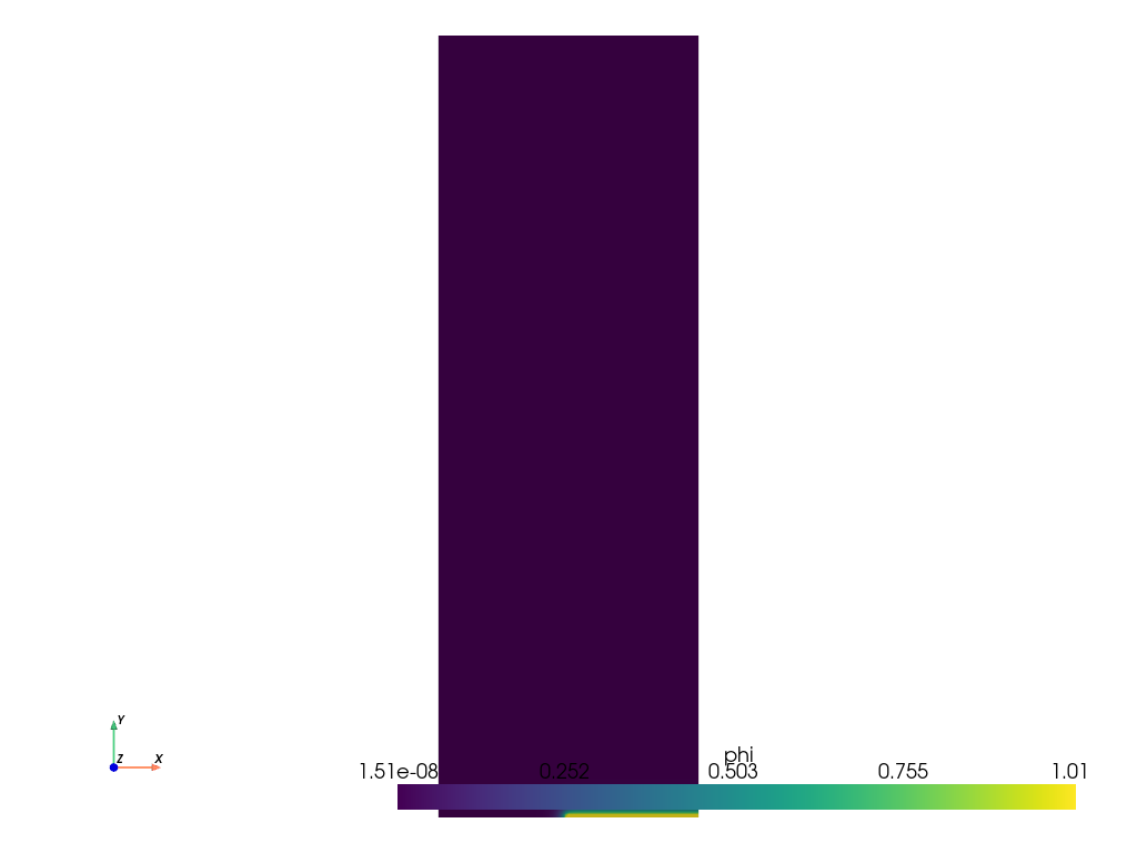
file_vtu = pv.read(os.path.join(Data.results_folder_name, "paraview-solutions_vtu", "phasefieldx_p0_000035.vtu"))
file_vtu.plot(scalars='phi', cpos='xy', show_scalar_bar=True, show_edges=False)
Plot: Displacement vs Fracture Energy#
force_quarter        = abs(S.reaction_files['bottom.reaction']["Ry"])
displacement_quarter = abs(2*S.energy_files['total.energy']["E"]/(S.reaction_files['bottom.reaction']["Ry"]))
stiffness_quarter    = abs(S.reaction_files['bottom.reaction']["Ry"]/displacement_quarter)
compliance_quarter   = 1/stiffness_quarter
dCda_quarter         = 2*Data.Gc/S.reaction_files['bottom.reaction']["Ry"]**2
gamma_quarter        = a0/2 + S.energy_files['total.energy']["gamma"]
lambda_quarter       = S.dof_files["lambda.dof"]["lambda"]
Complete model without corrections#
displacement_complete  = 2*displacement_quarter
force_complete         = 2*force_quarter
compliance_complete    = compliance_quarter
stiffness_complete     = stiffness_quarter
dCda_complete          = dCda_quarter/2.0
gamma_complete         = a0 + 2.0 * S.energy_files['total.energy']["gamma"]
gamma_phi_complete     = a0 + 2.0 * S.energy_files['total.energy']["gamma_phi"]
gamma_gradphi_complete = a0 + 2.0 * S.energy_files['total.energy']["gamma_gradphi"]


header = ["displacement", "force", "gamma", "compliance", "stiffness", "dCda"]
data_save = np.column_stack((displacement_complete, force_complete, gamma_complete, compliance_complete,stiffness_complete, dCda_complete))
save_path = os.path.join(Data.results_folder_name, "results.pff")
# np.savetxt(save_path, data_save, fmt="%.6e", delimiter="\t", header="\t".join(header), comments="")
Complete model with Gc corrections#
gc_factor = 1 + 2*h/(2*Data.l)
displacement_complete_corrected_gc  = displacement_complete/np.sqrt(gc_factor)
force_complete_corrected_gc         = force_complete/np.sqrt(gc_factor)
compliance_complete_corrected_gc    = compliance_complete
stiffness_complete_corrected_gc     = stiffness_complete
dCda_complete_corrected_gc          = dCda_complete*gc_factor
gamma_complete_corrected_gc         = a0 + 2.0 * S.energy_files['total.energy']["gamma"]/gc_factor
gamma_phi_complete_corrected_gc     = a0 + 2.0 * S.energy_files['total.energy']["gamma_phi"]/gc_factor
gamma_gradphi_complete_corrected_gc = a0 + 2.0 * S.energy_files['total.energy']["gamma_gradphi"]/gc_factor


header = ["displacement", "force", "gamma", "compliance", "stiffness", "dCda", "lambda"]
data_save = np.column_stack((displacement_complete_corrected_gc, force_complete_corrected_gc, gamma_complete_corrected_gc, compliance_complete_corrected_gc,stiffness_complete_corrected_gc, dCda_complete_corrected_gc))
save_path = os.path.join(Data.results_folder_name, "results_corrected_bourdin.pff")
# np.savetxt(save_path, data_save, fmt="%.6e", delimiter="\t", header="\t".join(header), comments="")
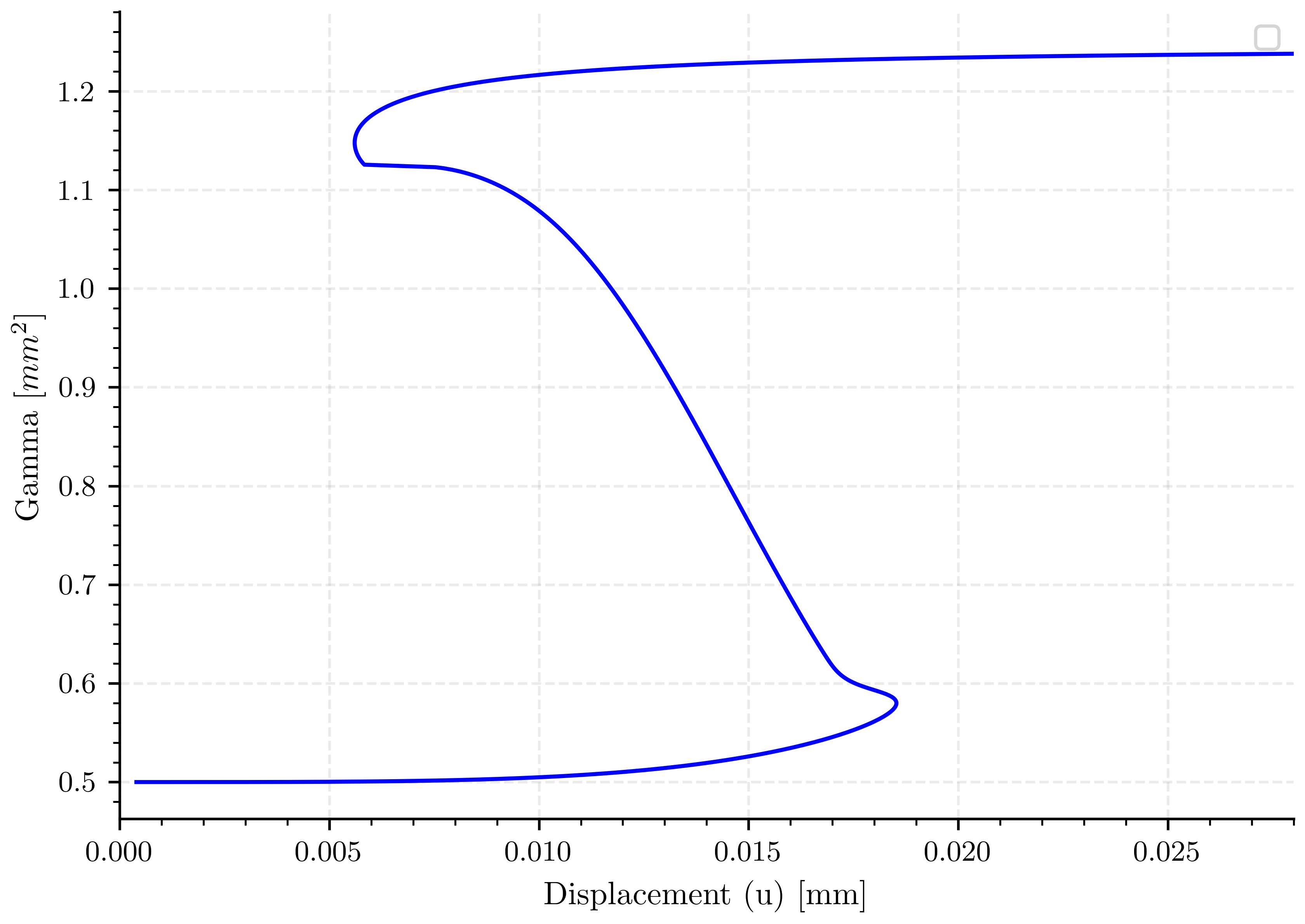
Plot: Force vs Vertical Displacement#
fig, energyg = plt.subplots()

energyg.plot(displacement_complete, gamma_complete, 'b-')
energyg.set_xlim(left=0.0, right=0.028)
energyg.set_xlabel(pcfg.displacement_label)
energyg.set_ylabel(pcfg.gamma_label)
energyg.legend()
/home/docs/checkouts/readthedocs.org/user_builds/phasefieldfatigue/checkouts/stable/examples/Phase_Field_Central_Cracked/plot_simulation_3_a05_l1.py:339: UserWarning: No artists with labels found to put in legend.  Note that artists whose label start with an underscore are ignored when legend() is called with no argument.
  energyg.legend()

<matplotlib.legend.Legend object at 0x734c56b33280>
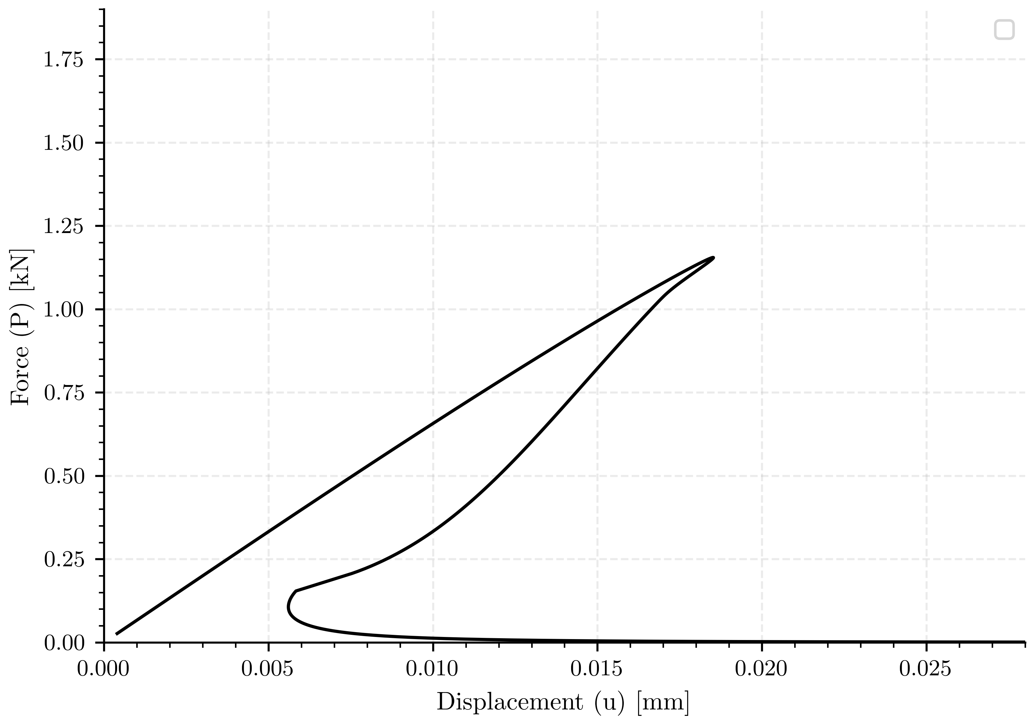
Plot: Force vs Vertical Displacement#
fig, ax_reaction = plt.subplots()

ax_reaction.plot(displacement_complete, force_complete, 'k-')

ax_reaction.set_xlim(left=0.0, right=0.028)
ax_reaction.set_ylim(bottom=0.0, top=1.9)
ax_reaction.set_xlabel(pcfg.displacement_label)
ax_reaction.set_ylabel(pcfg.force_label)
ax_reaction.legend()
/home/docs/checkouts/readthedocs.org/user_builds/phasefieldfatigue/checkouts/stable/examples/Phase_Field_Central_Cracked/plot_simulation_3_a05_l1.py:353: UserWarning: No artists with labels found to put in legend.  Note that artists whose label start with an underscore are ignored when legend() is called with no argument.
  ax_reaction.legend()

<matplotlib.legend.Legend object at 0x734c6385fd90>
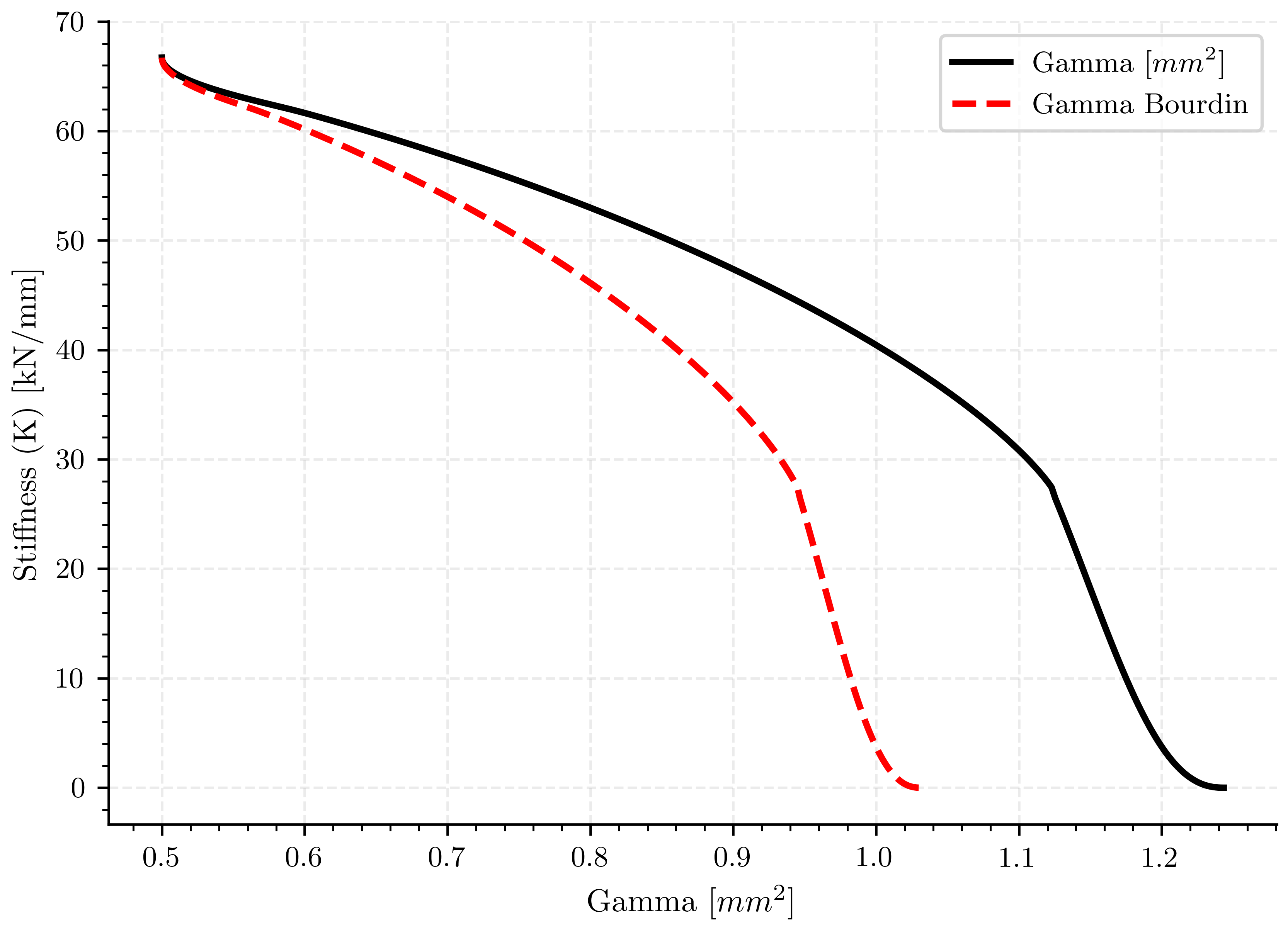
Plot: Force vs Vertical Displacement#
fig, ax_reaction = plt.subplots()

ax_reaction.plot(gamma_complete, stiffness_complete, 'k-', linewidth=2.0, label=pcfg.gamma_label)
ax_reaction.plot(gamma_complete_corrected_gc, stiffness_complete, 'r--', linewidth=2.0, label=pcfg.gamma_bourdin_label)

ax_reaction.set_xlabel(pcfg.gamma_label)
ax_reaction.set_ylabel(pcfg.stiffness_label)
ax_reaction.legend()

plt.show()
Total running time of the script: (0 minutes 5.357 seconds)