Fatigue Life Comparison: Simulation vs Experiment

This file presents a detailed comparison of fatigue life predictions for various compact specimen configurations, using the proposed simulation method and experimental results from Wagner[1].

The simulations compared are as follows:

Specimen configurations with varying initial crack positions (H) and hole presence.

Specimen	H (Crack Position)	Holes Considered
Specimen 1	\(H = 0.60 W = 24.0\) mm	No holes
Specimen 2	\(H = 0.56 W = 22.4\) mm	With holes
Specimen 3	\(H = 0.58 W = 23.2\) mm	With holes
Specimen 4	\(H = 0.64 W = 25.6\) mm	With holes

The experimental results used for comparison can be found in:

• Visualization of Experimental and Simulation Data from Wagner

This comparison highlights the agreement and differences in fatigue life predictions between the proposed simulation approach and experimental measurements.

[1]

D. Wagner. A finite element-based adaptive energy response function method for curvilinear progressive fracture. PhD thesis, The University of Texas at San Antonio, United States – Texas, 2018.

Import necessary libraries

import numpy as np
from scipy.integrate import cumulative_trapezoid
import matplotlib.pyplot as plt
import matplotlib.image as mpimg
import os
import shutil
import sys
import pandas as pd

sys.path.insert(0, os.path.abspath('../../'))
plt.style.use('../../graph.mplstyle')
import plot_config as pcfg

img = mpimg.imread('images/compact_specimen_holes.png')
plt.imshow(img)
plt.axis('off')

results_folder = "compact_phase_field"
if os.path.exists(results_folder):
    shutil.rmtree(results_folder)
os.makedirs(results_folder, exist_ok=True)

Load Results from Reference Paper

The experimental results are loaded below for comparison purposes. For more details, refer to the data in Visualization of Experimental and Simulation Data from Wagner.

paper_specimen_2 = pd.read_csv("../Papers_Data/Wagner_phd/specimen_a/experiment.paper", delim_whitespace=True)
paper_specimen_3 = pd.read_csv("../Papers_Data/Wagner_phd/specimen_b/experiment.paper", delim_whitespace=True)
paper_specimen_4 = pd.read_csv("../Papers_Data/Wagner_phd/specimen_c/experiment.paper", delim_whitespace=True)
color_papers_general = pcfg.color_grey
label_papers_general = r"Experiment"

Parameters definition

Define material and specimen parameters

E   = 211     # Young's modulus (kN/mm^2)
nu  = 0.3     # Poisson's ratio (-)
Gc  = 0.073   # Critical strain energy release rate (kN/mm)
Ep = E / (1.0 - nu**2) # Plane strain modulus (kN/mm^2)
# Coincide con R = 0.1
m = 2.08     # Paris' Law exponent (-)
Cparis = 1.615*10**(-8) * 10**(3*m/2)

Define specimen geometry

a0 = 8.0
W  = 40.0  # Characteristic width of the specimen (mm)
B  = 3.2   # Thickness (mm)

Ni = 0   # [cycles] Initial number of cycles
R = 0.1  # [-] Load ratio

theta = 0.04 # mm^-1
K0 = 15.0 * 1/(10*np.sqrt(10))
G0 = K0**2/(Ep)

Load the results

Here the results of all the specimen phase field simulation are loaded

label_pff_general = r"Phase-field"

The result form the specimen 1 without hole refering to the simulation Specimen 1. are loaded.

label_1 = r"specimen 1"
color_label_1 = pcfg.color_blue
results_1 = pd.read_csv("../Phase_Field_Compact_Specimen/results_specimen_1_H00/results_corrected_geometry.pff", delimiter="\t", comment="#", header=0)
a_1 = results_1["gamma"]
k_1 = 1/results_1["compliance"] * B
c_1 = results_1["compliance"] / B
dCda_1 = results_1["dCda"]/B
force_1 = results_1["force"] *B
u_1 = results_1["displacement"]

The result form the specimen 2 refering to the simulation Specimen 2. are loaded.

label_2 = r"specimen 2"
color_label_2 = pcfg.color_purple
results_2 = pd.read_csv("../Phase_Field_Compact_Specimen/results_specimen_2_H16/results_corrected_geometry.pff", delimiter="\t", comment="#", header=0)
a_2 = results_2["gamma"]
k_2 = 1/results_2["compliance"] * B
c_2 = results_2["compliance"] / B
dCda_2 = results_2["dCda"]/B
force_2 = results_2["force"] *B
u_2 = results_2["displacement"]

The result form the specimen 3 refering to the simulation Specimen 3. are loaded.

label_3 = r"specimen 3"
color_label_3 = pcfg.color_orangered
results_3 = pd.read_csv("../Phase_Field_Compact_Specimen/results_specimen_3_H08/results_corrected_geometry.pff", delimiter="\t", comment="#", header=0)
a_3 = results_3["gamma"]
k_3 = 1/results_3["compliance"] * B
c_3 = results_3["compliance"] / B
dCda_3 = results_3["dCda"]/B
force_3 = results_3["force"] *B
u_3 = results_3["displacement"]

The result form the specimen 4 without hole refering to the simulation Specimen 4. are loaded.

label_4 = r"specimen 4"
color_label_4 = pcfg.color_green
results_4 = pd.read_csv("../Phase_Field_Compact_Specimen/results_specimen_4_Hminus16/results_corrected_geometry.pff", delimiter="\t", comment="#", header=0)
a_4 = results_4["gamma"]
k_4 = 1/results_4["compliance"] * B
c_4 = results_4["compliance"] / B
dCda_4 = results_4["dCda"]/B
force_4 = results_4["force"] *B
u_4 = results_4["displacement"]

# Calculate marker frequency for each dataset
markevery_1 = max(1, len(u_1)//10)
markevery_2 = max(1, len(u_2)//10)
markevery_3 = max(1, len(u_3)//10)
markevery_4 = max(1, len(u_4)//10)

Crack length vs stiffness

The stiffness as function of crack length is plotted for all the specimens.

fig, ax0 = plt.subplots(figsize=(11.69, 5.85))  # A4 width in inches, half height for 2:1 aspect

# ax0.plot(a_1, k_1, color=color_label_1, linestyle='-', marker='o', markevery=10, label=label_1)
ax0.plot(a_1, k_1, color=color_label_1, linestyle='-', marker='o',
         markevery=markevery_1, label=label_1)
ax0.plot(a_2, k_2, color=color_label_2, linestyle='--', marker='s',
         markevery=markevery_2, label=label_2)
ax0.plot(a_3, k_3, color=color_label_3, linestyle='-', marker='^',
         markevery=markevery_3, label=label_3)
ax0.plot(a_4, k_4, color=color_label_4, linestyle='--', marker='D',
         markevery=markevery_4, label=label_4)

ax0.set_xlabel(pcfg.crack_length_label)
ax0.set_ylabel(pcfg.stiffness_label)
ax0.legend()

<matplotlib.legend.Legend object at 0x734c5e2b4d30>

Specimen 1: Force vs displacement

fig, ax_paper2 = plt.subplots()

ax_paper2.plot(u_1, force_1, color=color_label_1, linestyle='-', marker='o',
         markevery=markevery_1, label=label_1)

ax_paper2.set_ylabel(pcfg.force_label)
ax_paper2.set_xlabel(pcfg.displacement_label)
ax_paper2.set_xlim(left=-0.03, right=1.0)
ax_paper2.set_ylim(bottom=-1, top=22.3)

plt.savefig(os.path.join(results_folder,"force_displacement_specimen_1"))

Specimens 2,3,4: Force vs displacement

fig, ax_paper2 = plt.subplots()

ax_paper2.plot(u_2, force_2, color=color_label_2, linestyle='--', marker='s',
         markevery=markevery_2, label=label_2)
ax_paper2.plot(u_3, force_3, color=color_label_3, linestyle='-', marker='^',
         markevery=markevery_3, label=label_3)
ax_paper2.plot(u_4, force_4, color=color_label_4, linestyle='--', marker='D',
         markevery=markevery_4, label=label_4)

ax_paper2.set_ylabel(pcfg.force_label)
ax_paper2.set_xlabel(pcfg.displacement_label)
ax_paper2.set_xlim(left=-0.03, right=1.0)
ax_paper2.set_ylim(bottom=-1, top=22.3)
ax_paper2.legend()
plt.savefig(os.path.join(results_folder,"compare_force_displacement"))

Fatigue

Once the compliance curves are obtained, it is possible to calculate the fatigue lives from the compliance respect the crack area for the different methods.

def slice_array_by_values(a, value_1, value_2):
    """
    Returns a slice of the array `a` between the indices of the nearest values to `value_1` and `value_2`.

    Parameters:
    a (numpy.ndarray): The input array.
    value_1 (float): The first value to find in the array.
    value_2 (float): The second value to find in the array.

    Returns:
    numpy.ndarray: A new array sliced between the indices of the nearest values to `value_1` and `value_2`.
    """
    # Find the indices of the nearest values
    index_1 = (np.abs(a - value_1)).argmin()
    index_2 = (np.abs(a - value_2)).argmin()

    # Ensure index_1 is less than index_2
    if index_1 > index_2:
        index_1, index_2 = index_2, index_1

    # Return the sliced array
    return index_1, index_2 + 1

Slice the arrays to obtain the fatigue region

pre_crack = 3.5
a0_fatigue = 0.2*W + pre_crack # Initial crack length [mm]
i_o_1, i_f_1 = slice_array_by_values(a_1, a0_fatigue, max(a_1))
i_o_2, i_f_2 = slice_array_by_values(a_2, a0_fatigue, max(a_2))
i_o_3, i_f_3 = slice_array_by_values(a_3, a0_fatigue, max(a_3))
i_o_4, i_f_4 = slice_array_by_values(a_4, a0_fatigue, max(a_4))

a_fatigue_1, c_fatigue_1 = a_1[i_o_1:i_f_1], c_1[i_o_1:i_f_1]
a_fatigue_2, c_fatigue_2 = a_2[i_o_2:i_f_2], c_2[i_o_2:i_f_2]
a_fatigue_3, c_fatigue_3 = a_3[i_o_3:i_f_3], c_3[i_o_3:i_f_3]
a_fatigue_4, c_fatigue_4 = a_4[i_o_4:i_f_4], c_4[i_o_4:i_f_4]

dCda_fatigue_1 = dCda_1[i_o_1:i_f_1]
dCda_fatigue_2 = dCda_2[i_o_2:i_f_2]
dCda_fatigue_3 = dCda_3[i_o_3:i_f_3]
dCda_fatigue_4 = dCda_4[i_o_4:i_f_4]

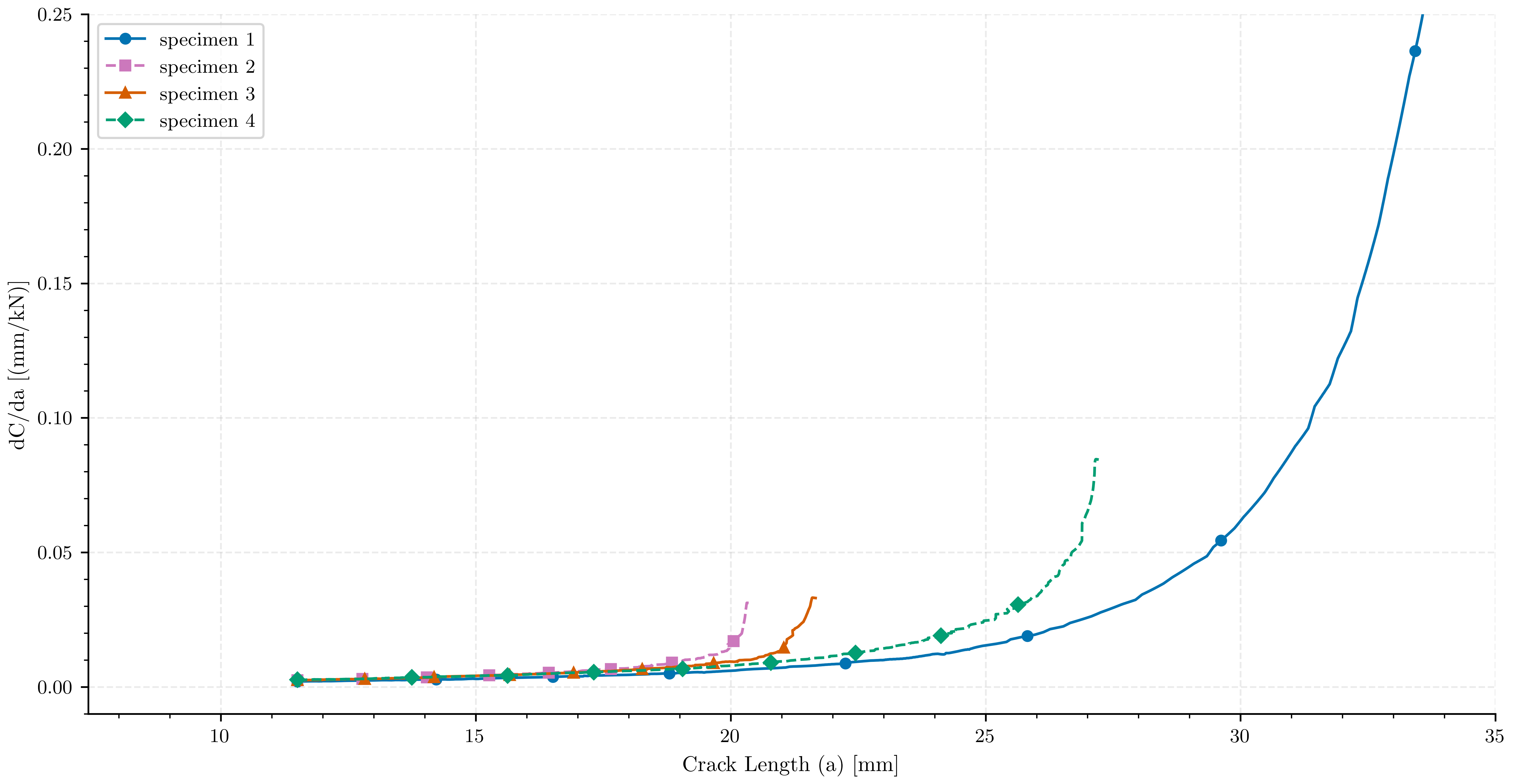
Crack length vs \(dC/da\)

The derivative of the compliance respect the crack area is plotted for the three methods.

fig, ax2 = plt.subplots(figsize=(11.69, 5.85))

ax2.plot(a_fatigue_1, dCda_fatigue_1, color=color_label_1, linestyle='-',
         marker='o', markevery=markevery_1, label=label_1)
ax2.plot(a_fatigue_2, dCda_fatigue_2, color=color_label_2, linestyle='--',
         marker='s', markevery=markevery_2, label=label_2)
ax2.plot(a_fatigue_3, dCda_fatigue_3, color=color_label_3, linestyle='-',
         marker='^', markevery=markevery_3, label=label_3)
ax2.plot(a_fatigue_4, dCda_fatigue_4, color=color_label_4, linestyle='--',
         marker='D', markevery=markevery_4, label=label_4)

ax2.set_xlabel(pcfg.crack_length_label)
ax2.set_ylabel(pcfg.dCda_label)
ax2.set_xlim(left=7.4, right=35.0)
ax2.set_ylim(bottom=-0.01, top=0.25)
ax2.legend()

<matplotlib.legend.Legend object at 0x734c54fb0670>

Once, the derivative of the compliance respect the crack area is calculated, it is possible to calculate the number of cycles to failure using the Paris law. In this case, the Paris law is used in the form:

\[N_f = N_i + \frac{1}{C (E'/2B)^{n/2} ((1-R) P_\text{max})^{n}} \int_{a_i}^{a_f} \frac{\mathrm{d}a}{(\mathrm{d}C/\mathrm{d}a)^{n/2} \ e^{n \theta(a-a_i)}}.\]

P_1 = np.sqrt(2*B*G0 / dCda_1[i_o_1])
P_2 = np.sqrt(2*B*G0 / dCda_2[i_o_2])
P_3 = np.sqrt(2*B*G0 / dCda_3[i_o_3])
P_4 = np.sqrt(2*B*G0 / dCda_4[i_o_4])

print(f"P_1: {P_1:.3f} kN")
print(f"P_2: {P_2:.3f} kN")
print(f"P_3: {P_3:.3f} kN")
print(f"P_4: {P_4:.3f} kN")

P_1: 1.746 kN
P_2: 1.574 kN
P_3: 1.558 kN
P_4: 1.533 kN

Calculate the number of cycles to failure for each method. The integration is performed using the trapezoidal rule.

Nf_dCda_1 = Ni + 1/(Cparis * (Ep/(2*B))**(m/2) * ((1-R)*P_1)**m)*cumulative_trapezoid(1/(dCda_fatigue_1)**(m/2) * 1/(np.exp(m*theta*(a_fatigue_1-a_1[i_o_1]))), a_fatigue_1, initial=0)
Nf_dCda_2 = Ni + 1/(Cparis * (Ep/(2*B))**(m/2) * ((1-R)*P_2)**m)*cumulative_trapezoid(1/(dCda_fatigue_2)**(m/2) * 1/(np.exp(m*theta*(a_fatigue_2-a_2[i_o_2]))), a_fatigue_2, initial=0)
Nf_dCda_3 = Ni + 1/(Cparis * (Ep/(2*B))**(m/2) * ((1-R)*P_3)**m)*cumulative_trapezoid(1/(dCda_fatigue_3)**(m/2) * 1/(np.exp(m*theta*(a_fatigue_3-a_3[i_o_3]))), a_fatigue_3, initial=0)
Nf_dCda_4 = Ni + 1/(Cparis * (Ep/(2*B))**(m/2) * ((1-R)*P_4)**m)*cumulative_trapezoid(1/(dCda_fatigue_4)**(m/2) * 1/(np.exp(m*theta*(a_fatigue_4-a_4[i_o_4]))), a_fatigue_4, initial=0)

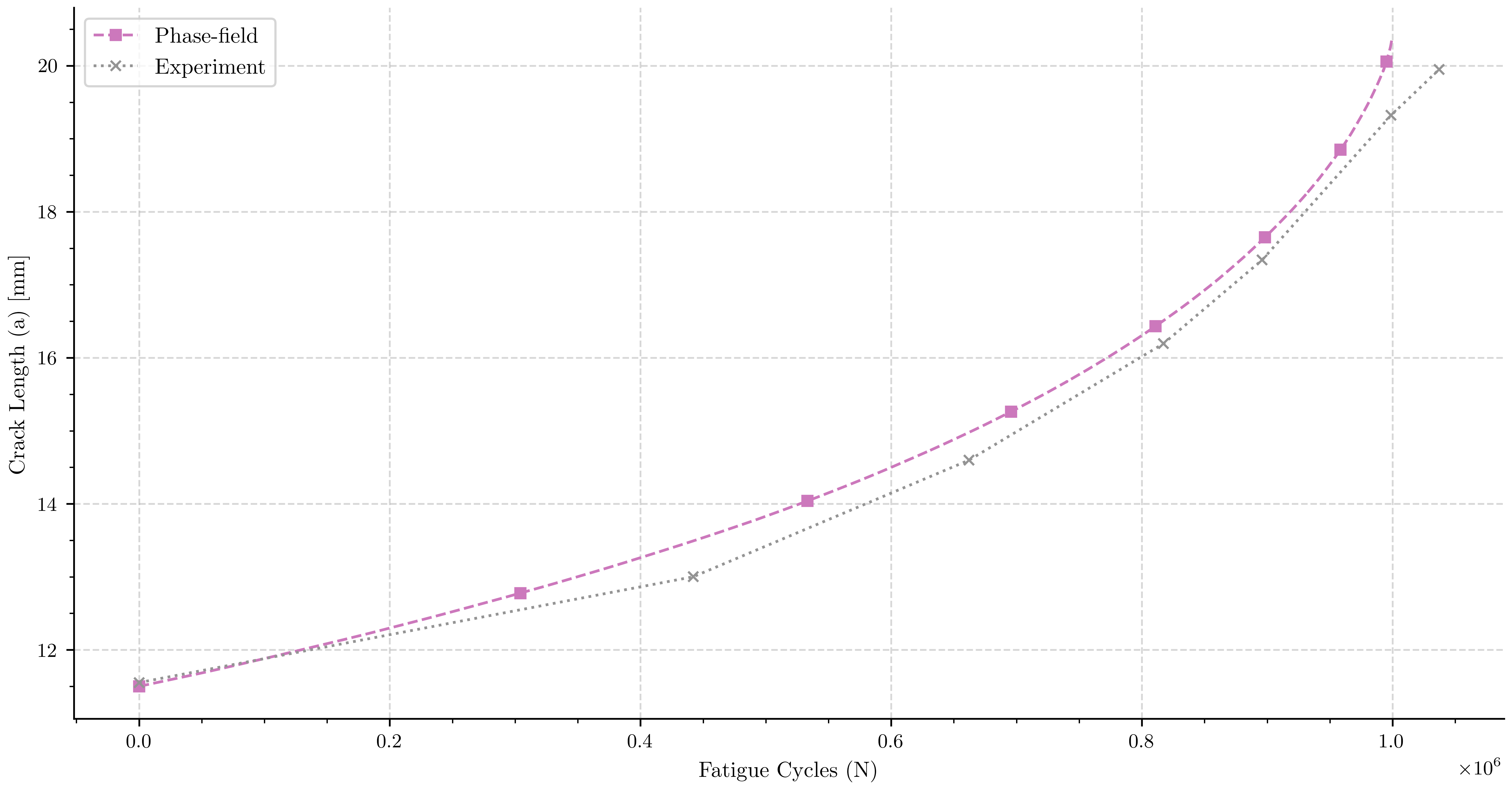
Individual comparison: Simulation vs Paper Specimen 2

fig, ax_paper2 = plt.subplots(figsize=(11.69, 5.85))
ax_paper2.plot(Nf_dCda_2, a_fatigue_2, color=color_label_2, linestyle='--',
               marker='s', markevery=markevery_2, label=label_pff_general)
ax_paper2.plot(paper_specimen_2["cycle_count"], paper_specimen_2["total_crack_length"], color=color_papers_general, linestyle=':', marker='x', label=label_papers_general)
ax_paper2.set_ylabel(pcfg.crack_length_label)
ax_paper2.set_xlabel(pcfg.cycles_label)
ax_paper2.legend(fontsize='medium', loc='best', frameon=True)
ax_paper2.grid(True, linestyle='--', alpha=0.5)
plt.savefig(os.path.join(results_folder, "compare_cycles_vs_crack_length_paper2"))

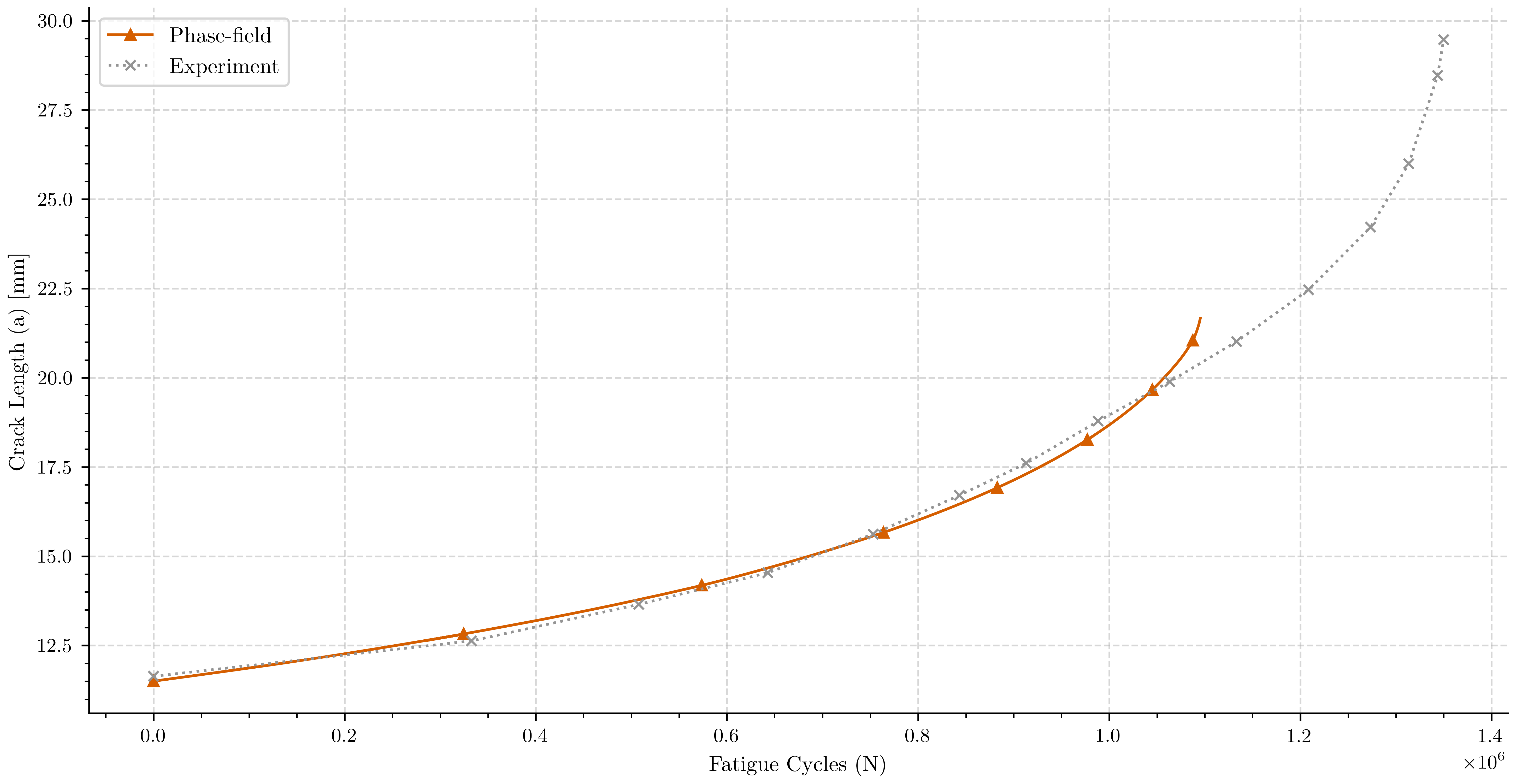
Individual comparison: Simulation vs Paper Specimen 3

fig, ax_paper3 = plt.subplots(figsize=(11.69, 5.85))
ax_paper3.plot(Nf_dCda_3, a_fatigue_3, color=color_label_3, linestyle='-',
               marker='^', markevery=markevery_3, label=label_pff_general)
ax_paper3.plot(paper_specimen_3["cycle_count"], paper_specimen_3["total_crack_length"], color=color_papers_general, linestyle=':', marker='x', label=label_papers_general)
ax_paper3.set_ylabel(pcfg.crack_length_label)
ax_paper3.set_xlabel(pcfg.cycles_label)
ax_paper3.legend(fontsize='medium', loc='best', frameon=True)
ax_paper3.grid(True, linestyle='--', alpha=0.5)
plt.savefig(os.path.join(results_folder, "compare_cycles_vs_crack_length_paper3"))

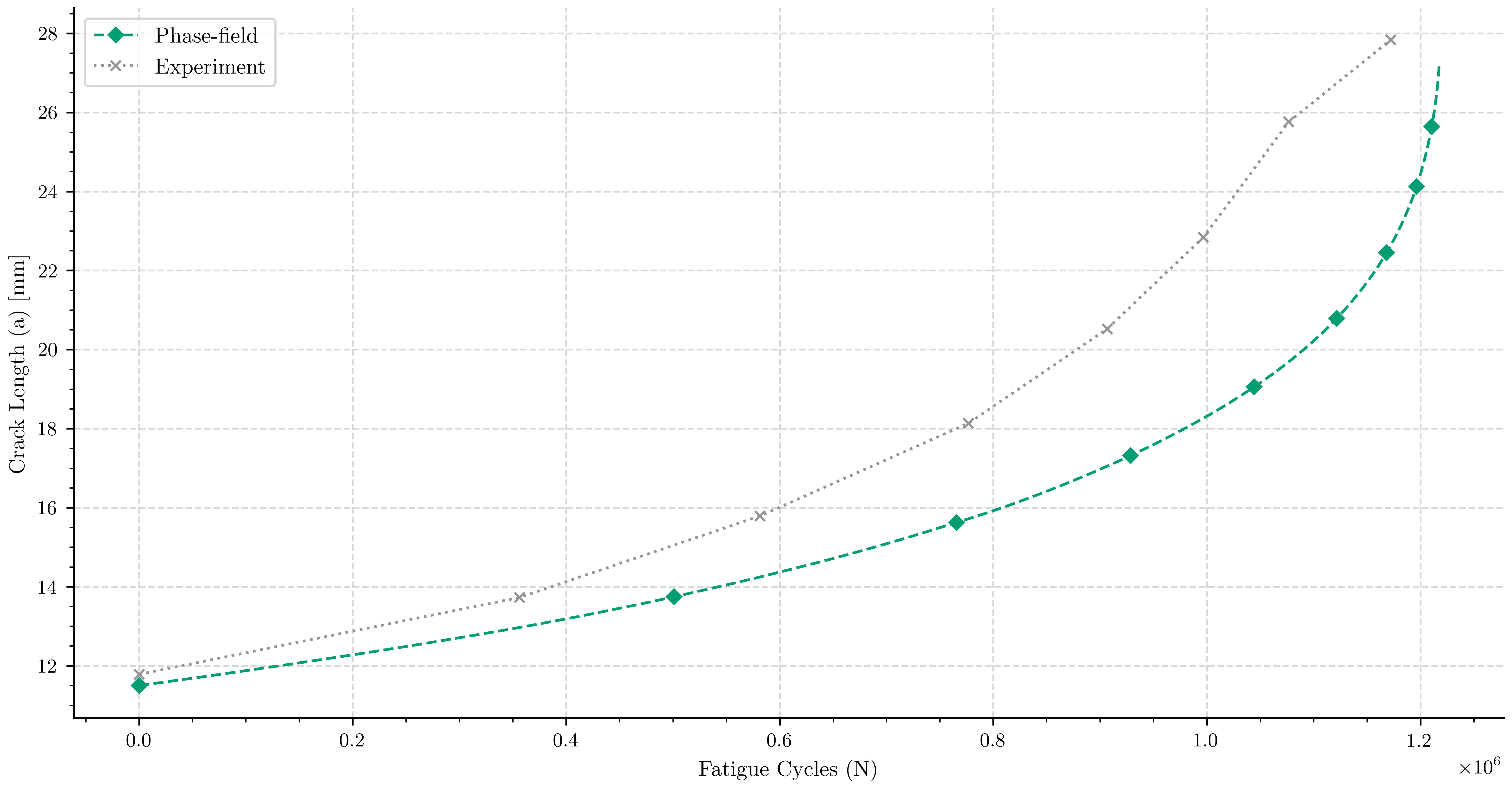
Individual comparison: Simulation vs Paper Specimen 4

fig, ax_paper4 = plt.subplots(figsize=(11.69, 5.85))
ax_paper4.plot(Nf_dCda_4, a_fatigue_4, color=color_label_4, linestyle='--',
               marker='D', markevery=markevery_4, label=label_pff_general)
ax_paper4.plot(paper_specimen_4["cycle_count"], paper_specimen_4["total_crack_length"], color=color_papers_general, linestyle=':', marker='x', label=label_papers_general)
ax_paper4.set_ylabel(pcfg.crack_length_label)
ax_paper4.set_xlabel(pcfg.cycles_label)
ax_paper4.legend(fontsize='medium', loc='best', frameon=True)
ax_paper4.grid(True, linestyle='--', alpha=0.5)
plt.savefig(os.path.join(results_folder, "compare_cycles_vs_crack_length_paper4"))

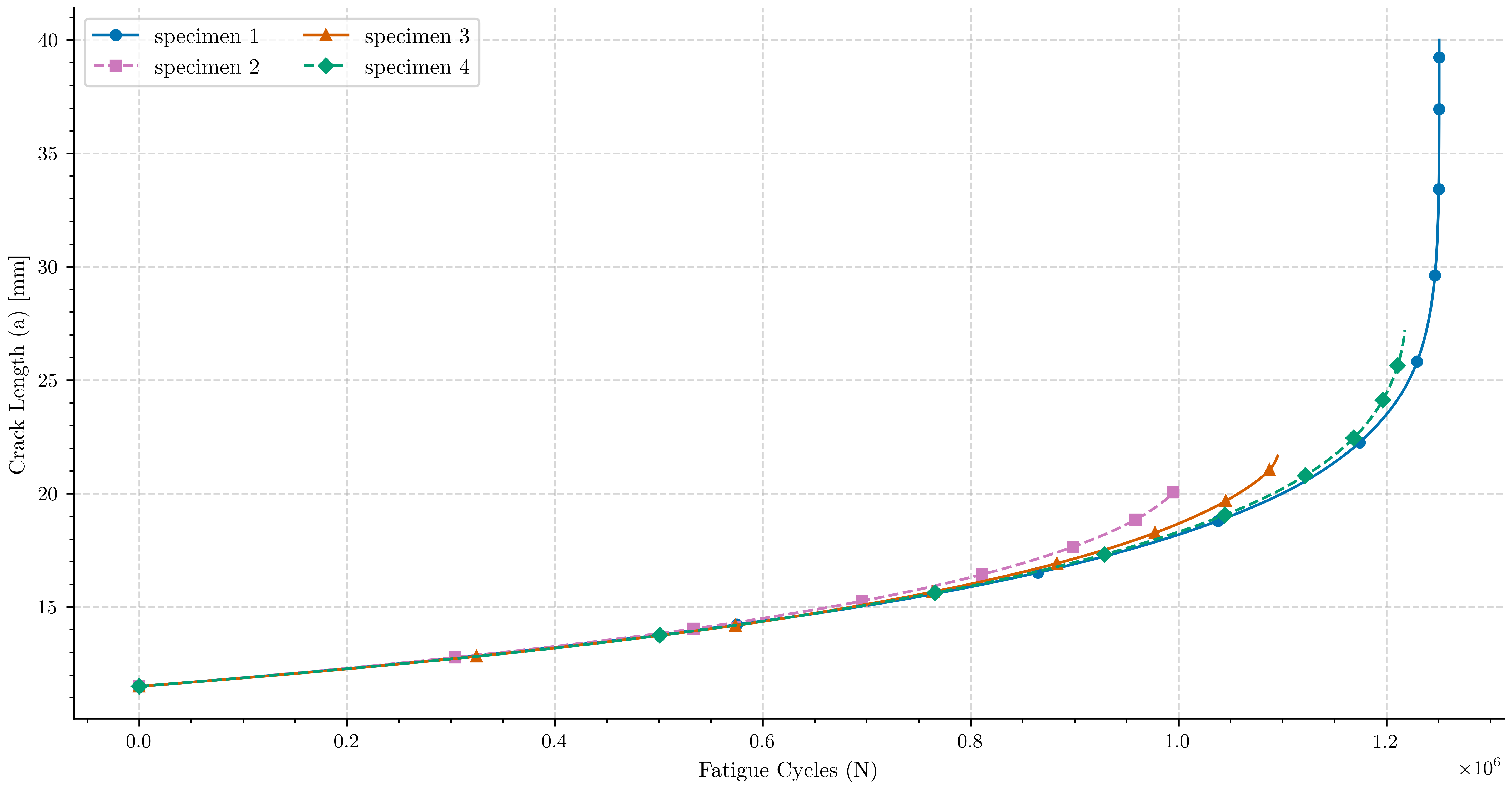
Crack length vs number of cycles

The number of cycles to failure is calculated from the compliance respect the crack length for the different methods.

fig, ax3 = plt.subplots(figsize=(11.69, 5.85))  # Match previous plot size for consistency

# Plot your simulation results
ax3.plot(Nf_dCda_1, a_fatigue_1, color=color_label_1, linestyle='-',
         marker='o', markevery=markevery_1, label=label_1)
ax3.plot(Nf_dCda_2, a_fatigue_2, color=color_label_2, linestyle='--',
         marker='s', markevery=markevery_2, label=label_2)
ax3.plot(Nf_dCda_3, a_fatigue_3, color=color_label_3, linestyle='-',
         marker='^', markevery=markevery_3, label=label_3)
ax3.plot(Nf_dCda_4, a_fatigue_4, color=color_label_4, linestyle='--',
         marker='D', markevery=markevery_4, label=label_4)


# Enhance plot aesthetics for visual comparison
ax3.set_ylabel(pcfg.crack_length_label)
ax3.set_xlabel(pcfg.cycles_label)
ax3.legend(ncol=2, fontsize='medium', loc='best', frameon=True)
ax3.grid(True, linestyle='--', alpha=0.5)

plt.savefig(os.path.join(results_folder, "paper_compare_cycles_vs_crack_length"))

plt.show()


# Calculate percentage difference for each simulation vs experiment
percent_diff_2 = 100 * abs(Nf_dCda_2[-1] - paper_specimen_2["cycle_count"].iloc[-1]) / paper_specimen_2["cycle_count"].iloc[-1]
percent_diff_3 = 100 * abs(Nf_dCda_3[-1] - paper_specimen_3["cycle_count"].iloc[-1]) / paper_specimen_3["cycle_count"].iloc[-1]
percent_diff_4 = 100 * abs(Nf_dCda_4[-1] - paper_specimen_4["cycle_count"].iloc[-1]) / paper_specimen_4["cycle_count"].iloc[-1]

print(f"Percentage difference Specimen 2: {percent_diff_2:.2f}%")
print(f"Percentage difference Specimen 3: {percent_diff_3:.2f}%")
print(f"Percentage difference Specimen 4: {percent_diff_4:.2f}%")

Percentage difference Specimen 2: 3.65%
Percentage difference Specimen 3: 18.87%
Percentage difference Specimen 4: 3.88%