Note
Go to the end to download the full example code.
Specimen 1#
This example demonstrates the procedure for generating a mesh for the compact tension specimen presented in Wagner[1], from which some of the simulation results will be compared. In this case, the mesh refers to the configuration with no additional holes, so the dimensions of the mesh are related to the stress intensity factor presented in Anderson[2] and Tada[3].
All dimensions follow the relationship given in the LEFM formula, which refers to the base dimension \(b\). In the case of the paper, \(b = 40\) mm, but with this script, the geometry can be scaled simply by modifying this value in the .geo file.
Below is the .geo file used for the specimen 1:
Reference#
// -----------------------------------------------------------------------------
//
// Gmsh GEO: Specimen 1
// ====================
//
// -----------------------------------------------------------------------------
//
// Use the following line to generate the mesh:
// gmsh specimen_1_H00.geo -2 -o specimen_1_H00.msh
//
//      *------------------------------------* -
//      |                                    | |
//      |  _  /-----\                        | |
//      |  | |       |                       | |
//    - | D| |       |                       | |
//    | |  | |       |                       | | hg
//    | |  -  \-----/                        | |
//  h1| |                                    | |
//    | |      (0,0)                         | |
//    -  --------*------                     | -
//    | |                                    | |
//  h1| |                                    | |
//    | |  _  /-----\                        | |
//    | |  | |       |                       | | hg
//    - | D| |       |                       | |
//      |  | |       |                       | |
//      |  -  \-----/                        | |
//      |                                    | |
//      *------------------------------------* -
//                |--a--|
//      |---c-----|-------------b------------|
//
// +---------------+---------------+
// | Parameter     | Value         |
// +===============+===============+
// | $hg$          | $0.6 b$       |
// +---------------+---------------+
// | $h1$          | $0.275 b$     |
// +---------------+---------------+
// | $D$           | $0.25 b$      |
// +---------------+---------------+
// | $c$           | $0.25 b$      |
// +---------------+---------------+

H = 0.0;
b = 40.0;

// Mesh size parameters
// --------------------
h      = (0.04)*b;  // mesh size far from the crack
hcrack = (0.002)*b; //mesh size near crack


// Parameters for the geometry
// ---------------------------
// All the parameters are defined in terms of the base length "b"
// Change the value of "b" to scale the geometry
hg = (0.6)*b;
a  = (0.2)*b;
h1 = (0.275)*b;
c  = (0.25)*b;
D  = (0.25)*b;


//           |
//           |
//   -       |   *
//   |       | / |
//   |  -    *   |
//  j|  |        |
//   | f|  -     *---------------*\
//   |  | l|                       \
//   -  -  - |---|             30º  \  (a,H)
//             k            -.-.-.-. *
//                                  /
//                                 /
//               *---------------*/
//               |*
//           *   |
//           | \ |
//           |   *
//           |
//           |
f = (0.06375)*b;
j = (0.08875)*b;
k = (0.04250)*b;
l = (0.00375)*b;

angle_deg = 30;
angle_rad = angle_deg * Pi / 180;
tan30 = Tan(angle_rad);
g = a - (l/tan30);

SetFactory("OpenCASCADE");

// ------------------------------------------------------
// ------------------------------------------------------
// A)Geometry Definition: 1)Points
//                        2)Lines
//                        3)Curve
//                        4)Surface

// ------------------------------------------------------
// A1)Points Definitions:
//
//         P4*----------------------*P3
//           |                      |
//           |                      |
//           |                      |
//           |   *P6                |
//           | / |                  |
//         P5*   |                  |
//               |P7     P8         |
//               *-------*\         |
//                         \        |
//                          *P9     |
//                         /        |
//               *-------*/         |
//               |*P11  P10         |
//        P13*   |                  |
//           | \ |                  |
//           |   *P12               |
//           |                      |
//           |                      |
//           |                      |
//           |                      |
//         P1*---------------------*P2
//
//    |Y
//    |
//    ---X
//

//           --Coordinates--
//Points:    -------X,------Y,--Z,
Point(1)   = {     -c,    -hg,  0,  h};
Point(2)   = {      b,    -hg,  0,  h};
Point(3)   = {      b,     hg,  0,  h};
Point(4)   = {     -c,     hg,  0,  h};
Point(5)   = {     -c,    H+f,  0,  h};
Point(6)   = {   -c+k,    H+j,  0,  h};
Point(7)   = {   -c+k,    H+l,  0,  h};
Point(8)   = {      g,    H+l,  0,  h};
Point(9)   = {      a,      H,  0,  h};
Point(10)  = {      g,    H-l,  0,  h};
Point(11)  = {   -c+k,    H-l,  0,  h};
Point(12)  = {   -c+k,    H-j,  0,  h};
Point(13)  = {     -c,    H-f,  0,  h};


// ------------------------------------------------------
// A2)Lines Definition
Line(1) = {1, 2};  //L1:from P1 to P2: P1*--L1-->*P2
Line(2) = {2, 3};
Line(3) = {3, 4};
Line(4) = {4, 5};
Line(5) = {5, 6};
Line(6) = {6, 7};
Line(7) = {7, 8};
Line(8) = {8, 9};
Line(9) = {9, 10};
Line(10) = {10, 11};
Line(11) = {11, 12};
Line(12) = {12, 13};
Line(13) = {13, 1};

// ------------------------------------------------------
// A3)Curve Definition
//
Curve Loop(5) = {1,2,3,4,5,6,7,8,9,10,11,12,13};  //C5: through lines L1,L2,...,L7

// The following curves represent the circles and arcs in the geometry
//
//      *------------------------------------*
//      |                                    |
//      |     /-----\                        |
//      |    |       |                       |
//      | P16*  *P14 *P15                    |
//      |    |       |                       |
//      |     \-----/                        |
//      |                                    |
//      |      (0,0)                         |
//       --------*------                     |
//      |                                    |
//      |                                    |
//      |     /-----\                        |
//      |    |       |                       |
//      | P19*  *P17 *P18                    |
//      |    |       |                       |
//      |     \-----/                        |
//      |                                    |
//      *------------------------------------*

// Top circle -------------------------------------------------
Point(14) = {       0, h1, 0, h};   // Center of the circle
Point(15) = { (D)*0.5, h1, 0, h};   // Start point
Point(16) = {(-D)*0.5, h1, 0, h};   // End point of the first arc

Circle(100) = {15, 14, 16};  // First half of the circle
Circle(101) = {16, 14, 15};  // Second half of the circle

Curve Loop(200) = {100, 101};

// Bottom circle -----------------------------------------------
//
Point(17) = {        0, -h1, 0, h};   // Center of the circle
Point(18) = {  (D)*0.5, -h1, 0, h};   // Start point
Point(19) = { (-D)*0.5, -h1, 0, h};   // End point of the first arc

Circle(102) = {18, 17, 19};  // First half of the circle
Circle(103) = {19, 17, 18};  // Second half of the circle

Curve Loop(201) = {102, 103};


// ------------------------------------------------------
// A4)Surface Definition
//
//        *----------*
//        |          |
//        *  \       |
//            *  S6  |
//        *  /       |
//        |          |
//        *----------*
//
Plane Surface(6) = {5, 200, 201};  // Subtract circle loops the main surface
Recombine Surface {6};

// Extrude the Surfaces to Create the Volumes
// Extrude {0.0, 0.0, thickness}{Surface{6};}

// ------------------------------------------------------
// ------------------------------------------------------
// B)Mesh Generation: 1)Mesh size Box1
//                    2)Mesh size Box2
//                    3)Mesh min(Box1,Box2)
//                    3)Extrude Mesh
//                    4)Mesh Algorithm


// ------------------------------------------------------
// B1) Mesh size Box1
//
//        *----------------*
//        |  / - \         |
//        |  |   | (Field[6])
//        |  \ - /         |
//         -----------     |
//        |                |
//        |                |
//        |                |
//        *----------------*

Field[6] = Attractor;
Field[6].EdgesList = {101};

// Define a Threshold field to control mesh size near the attractor
Field[66] = Threshold;
Field[66].InField = 6;         // Use the Attractor field
Field[66].SizeMin = hcrack;    // Minimum mesh size near the attractor
Field[66].SizeMax = h;         // Maximum mesh size far from the attractor
Field[66].DistMin = 0.00;      // Distance from the attractor where SizeMin is applied
Field[66].DistMax = 0.25;       // Distance from the attractor where SizeMax is applied


// ------------------------------------------------------
// B2) Mesh size Box2
//
//        *----------------*
//        |                |
//        |                |
//        |                |
//         -----------     |
//        |  / - \         |
//        |  |   | (Field[7])
//        |  \ - /         |
//        *----------------*
Field[7] = Attractor;
Field[7].EdgesList = {102};

// Define a Threshold field to control mesh size near the attractor
Field[77] = Threshold;
Field[77].InField = 7;         // Use the Attractor field
Field[77].SizeMin = hcrack;    // Minimum mesh size near the attractor
Field[77].SizeMax = h;         // Maximum mesh size far from the attractor
Field[77].DistMin = 0.00;      // Distance from the attractor where SizeMin is applied
Field[77].DistMax = 0.25;      // Distance from the attractor where SizeMax is applied

// ------------------------------------------------------
// B3) Mesh size Box3
//
//        *----------------*
//        |                |
//        |                |
//        |                |
//        *     -----------|
//             | (Field[8])|
//        *     -----------|
//        |                |
//        |                |
//        |                |
//        *----------------*
Field[8]      =    Box;
Field[8].VIn  = hcrack;
Field[8].VOut =      h;

Field[8].XMin =  g;
Field[8].XMax =  b;
Field[8].YMin = -0.04*b;
Field[8].YMax =  0.04*b;


// ------------------------------------------------------
// B3) Mesh min(Box1,Box2)
Field[14] = Min;
Field[14].FieldsList = {8, 66, 77};
Background Field = 14;


// ------------------------------------------------------
// B5)Mesh Algorithm
Geometry.Tolerance = 1e-12;
// Mesh.Algorithm = 1;
Mesh.Algorithm = 8;                    // Frontal-Delaunay for quads
Mesh.RecombineAll = 1;                 // Recombine all surfaces
Mesh.SubdivisionAlgorithm = 1;         // All quads subdivision
Mesh.RecombinationAlgorithm = 1;       // Simple recombination
// ------------------------------------------------------
// Physical groups definition
//

Physical Surface("surface", 202) = {6};

Physical Curve("circle_top_top", 204) = {101};
Physical Curve("circle_top_bottom", 205) = {100};

Physical Curve("circle_bottom_top", 206) = {103};
Physical Curve("circle_bottom_bottom", 203) = {102};
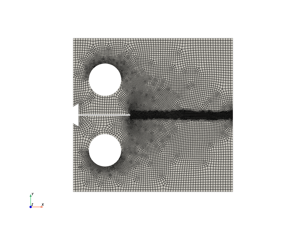
Mesh Visualization#
The purpose of this code is to visualize the mesh. The mesh is generated from the .geo file and saved as output_mesh_for_view.vtu. It is then loaded and visualized using PyVista.
import os
import gmsh
import pyvista as pv

folder = "Compact_specimen"
Reference#
Initialize Gmsh
gmsh.initialize()
Open the .geo file
geo_file = os.path.join(folder, "specimen_1_H00.geo")
gmsh.open(geo_file)
Generate the mesh (2D example, for 3D use generate(3))
gmsh.model.mesh.generate(2)
Write the mesh to a .vtk file for visualization Note that the input mesh file for the phasefieldx simulation should have the .msh extension. Use “output_mesh_for_view.msh” to generate the mesh for the simulation input. In this case, the mesh is saved in .vtk format to facilitate visualization with PyVista.
vtu_file = os.path.join(folder, "output_mesh_for_view_1.vtk")
gmsh.write(vtu_file)
Finalize Gmsh
gmsh.finalize()

print(f"Mesh successfully written to {vtu_file}")

pv.start_xvfb()
file_vtu = pv.read(vtu_file)
file_vtu.plot(cpos='xy', color='white', show_edges=True)

save_image=False
# Create a PyVista plotter
if save_image:
   plotter = pv.Plotter(off_screen=True)

   # Add the mesh with a light gray surface and visible edges
   plotter.add_mesh(file_vtu, color="lightgray", show_edges=True,
                         edge_color="darkblue", line_width=0.5, opacity=0.7)

   # Add the wireframe with darker lines to highlight the mesh structure
   plotter.add_mesh(file_vtu, style="wireframe", color="black",
                         line_width=1.2)

   # Set the view and background
   plotter.view_xy()
   plotter.set_background("white")
   plotter.camera.tight(padding=0.0)
   plotter.camera.clipping_range = (0.1, 1000.0)

   # Save the screenshot
   image_file = os.path.join(folder, "specimen_1_H00.png")
   plotter.screenshot(image_file, transparent_background=False, return_img=False)
   plotter.close()

   print(f"Image saved to {image_file}")
Mesh successfully written to Compact_specimen/output_mesh_for_view_1.vtk
Total running time of the script: (0 minutes 6.350 seconds)