Note
Go to the end to download the full example code.
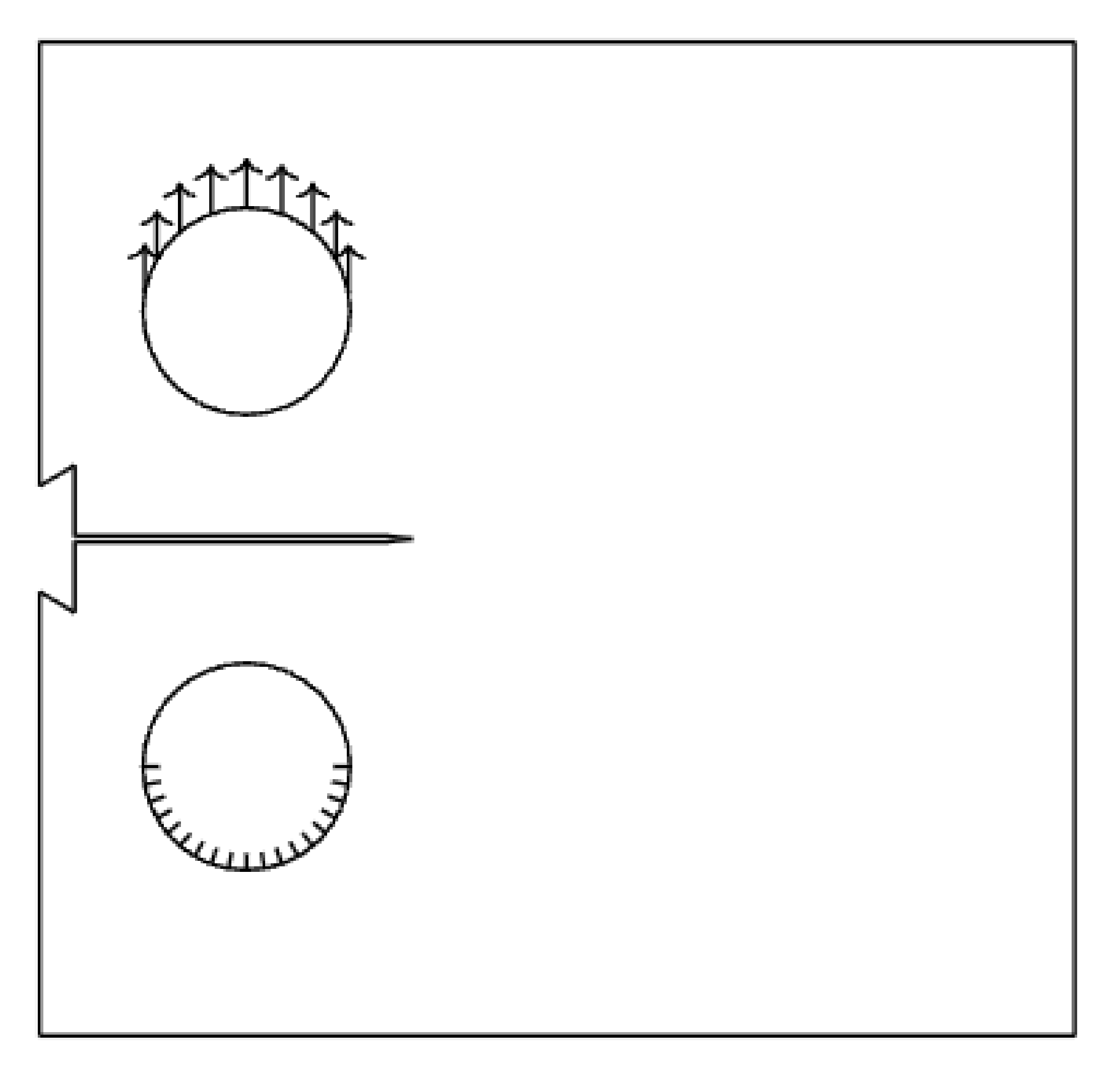
Force Controlled Compact Specimen#
This section presents several analyses conducted using specific meshes tailored for each case. The boundary conditions are carefully defined to ensure accurate representation of the physical behavior of the compact tension specimen under force-controlled loading.
#
#       *----------------* -
#       |                |
#       |                |
#     - |   /.\          | | h
#   h1| |   \ /          | |
#     | |                | |
#     -  ----------      | -
#     | |        _       | |
#   h1| |   / \  |       | | h
#     - |   \./  | D     | |
#       |        -       | |
#       |              | |
#       *----------------* -
#            |--a--|
#       |-c--|-----b-----|
#
#
#  +---------------+---------------+
#  | Parameter     | Value         |
#  +===============+===============+
#  | $h$           | $0.6 b$       |
#  +---------------+---------------+
#  | $h1$          | $0.275 b$     |
#  +---------------+---------------+
#  | $D$           | $0.25 b$      |
#  +---------------+---------------+
#  | $c$           | $0.25 b$      |
#  +---------------+---------------+
#
The Young’s modulus, Poisson’s ratio, and the critical energy release rate are given in the table Properties. Young’s modulus \(E\) and Poisson’s ratio \( u\) can be represented with the Lamé parameters as: \(\lambda= rac{E u}{(1+ u)(1-2 u)}\); \(\mu= rac{E}{2(1+ u)}\).
Material Properties#
The material properties are summarized in the table below:
VALUE |
UNITS |
|
|---|---|---|
E |
211 |
kN/mm2 |
nu |
0.3 |
[-] |
Import necessary libraries#
import numpy as np
import matplotlib.pyplot as plt
import matplotlib.image as mpimg
import pyvista as pv
import pandas as pd
import dolfinx
import mpi4py
import petsc4py
import os
import sys

sys.path.insert(0, os.path.abspath('../../'))
plt.style.use('../../graph.mplstyle')
import plot_config as pcfg

img = mpimg.imread('images/compact_specimen.png')  # or .jpg, .tif, etc.
plt.imshow(img)
plt.axis('off')
(-0.5, 387.5, 372.5, -0.5)
Import from phasefieldx package#
from phasefieldx.Element.Elasticity.Input import Input
from phasefieldx.Element.Elasticity.solver.solver import solve
from phasefieldx.Boundary.boundary_conditions import bc_xy, bc_y, get_ds_bound_from_marker
from phasefieldx.Loading.loading_functions import loading_Txy
from phasefieldx.PostProcessing.ReferenceResult import AllResults


results_folder = "results_compact_tension_gmsh"
if not os.path.exists(results_folder):
    os.makedirs(results_folder)

def run_simulations(i, msh_file):
    Data = Input(E=211.0,
                 nu=0.3,
                 save_solution_xdmf=False,
                 save_solution_vtu=True,
                 results_folder_name=os.path.join(results_folder,str(i)))


    ###############################################################################
    # Mesh Definition
    # ---------------
    # The mesh is generated using Gmsh and saved as a 'mesh.msh' file. For more details
    # on how to create the mesh, refer to the :ref:`ref_example_geo_gomes` examples.
    # msh_file = os.path.join("mesh.msh")  # Path to the mesh file
    gdim = 2                                    # Geometric dimension of the mesh
    gmsh_model_rank = 0                        # Rank of the Gmsh model in a parallel setting
    mesh_comm = mpi4py.MPI.COMM_WORLD            # MPI communicator for parallel computation

    # %%
    # The mesh, cell markers, and facet markers are extracted from the 'mesh.msh' file
    # using the `read_from_msh` function.
    msh, cell_markers, facet_markers = dolfinx.io.gmshio.read_from_msh(msh_file, mesh_comm, gmsh_model_rank, gdim)

    fdim = msh.topology.dim - 1 # Dimension of the mesh facets

    # %%
    # Facets defined in the .geo file used to generate the 'mesh.msh' file are identified here.
    # Each marker variable corresponds to a specific region on the specimen:
    #
    # - `bottom_facet_marker`: Refers to the bottom part of the specimen.
    # - `top_facet_marker`: Refers to the top part of the specimen.
    # - `right_facet_marker`: Refers to the right side of the specimen.
    # - `left_facet_marker`: Refers to the left side of the specimen.

    top_top_facet_marker = facet_markers.find(204)
    top_bottom_facet_marker = facet_markers.find(205)

    bottom_top_facet_marker    = facet_markers.find(206)
    bottom_bottom_facet_marker = facet_markers.find(203)


    ds_top = get_ds_bound_from_marker(top_top_facet_marker, msh, fdim)
    ds_bottom = get_ds_bound_from_marker(bottom_bottom_facet_marker, msh, fdim)


    ds_list = np.array([
                    [ds_top, "top"],
                    [ds_bottom, "bottom"],
                    ])


    V_u = dolfinx.fem.functionspace(msh, ("Lagrange", 1, (msh.geometry.dim, )))

    bc_bottom_bottom = bc_xy(bottom_bottom_facet_marker, V_u, fdim)
    bc_bottom_top    = bc_xy(bottom_top_facet_marker, V_u, fdim)
    bcs_list_u = [bc_bottom_bottom]
    bcs_list_u_names = ["bottom_bottom"]


    def update_boundary_conditions(bcs, time):
        return 0, 0, 0

    ###############################################################################
    # External Load Definition
    # ------------------------
    # Here, we define the external load to be applied to the top boundary (`ds_top`).
    # `T_top` represents the external force applied in the y-direction.
    surface_aplication_force = np.pi*16 /2
    T_top = dolfinx.fem.Constant(msh, petsc4py.PETSc.ScalarType((0.0, 1.0/surface_aplication_force)))


    # %%
    # The load is added to the list of external loads, `T_list_u`, which will be updated
    # incrementally in the `update_loading` function.
    T_list_u = [[T_top, ds_top]
            ]
    f = None

    ###############################################################################
    # Function: `update_loading`
    # --------------------------
    # The `update_loading` function is responsible for incrementally applying an external load at each
    # time step, achieving a force-controlled quasi-static loading. This function allows for gradual
    # increase in force along the y-direction on a specific boundary facet, simulating controlled
    # force application over time.
    #
    # Parameters:
    #
    # - `T_list_u`: List of tuples where each entry corresponds to a load applied to a specific
    #   boundary or facet of the mesh.
    # - `time`: Scalar representing the current time step in the analysis.
    #
    # Inside the function:
    #
    # - `val` is calculated as `0.1 * time`, a linear function of `time`, which represents the
    #   gradual application of force in the y-direction. This scaling factor (`0.1` in this case) can
    #   be adjusted to control the rate of force increase.
    # - The value `val` is assigned to the y-component of the external force field on the top boundary
    #   by setting `T_list_u[0][0].value[1]`, where `T_list_u[0][0]` represents the load applied to
    #   the designated top boundary facet (`ds_top`).
    #
    # Returns:
    #
    # - A tuple `(0, val, 0)` where:
    # - The first element is zero, indicating no load in the x-direction.
    # - The second element is `val`, the calculated y-directional force.
    # - The third element is zero, as this is a 2D example without z-component loading.
    #
    # This function supports force-controlled quasi-static analysis by adjusting the applied load
    # over time, ensuring a controlled force increase in the simulation.
    def update_loading(T_list_u, time):
        val = 1.0
        T_list_u[0][0].value[1] = petsc4py.PETSc.ScalarType(val)
        return 0, val, 0

    f = None

    final_time = 1.0
    dt = 1.0

    solve(Data,
        msh,
        final_time,
        V_u,
        bcs_list_u,
        update_boundary_conditions,
        f,
        T_list_u,
        update_loading,
        ds_list,
        dt,
        path=None,
        quadrature_degree=2,
        bcs_list_u_names=bcs_list_u_names)

mesh_folders = "../GmshGeoFiles/combo/generated_meshes"


import os
import glob
import re

def get_ordered_msh_files(folder_path):
    """
    Get ordered list of .msh files from a folder.

    Parameters:
    -----------
    folder_path : str
        Path to the folder containing .msh files

    Returns:
    --------
    list : Ordered list of full paths to .msh files
    """
    # Get all .msh files
    msh_files = glob.glob(os.path.join(folder_path, "*.msh"))

    # Sort naturally (handles numbers correctly)
    msh_files.sort(key=lambda x: [int(c) if c.isdigit() else c.lower()
                                  for c in re.split('([0-9]+)', os.path.basename(x))])

    return msh_files

# Usage in your code:
mesh_files = get_ordered_msh_files(mesh_folders)

print(f"Found {len(mesh_files)} mesh files:")
for i, file in enumerate(mesh_files):
    print(f"  {i}: {os.path.basename(file)}")

run_simulation_bool = False

if run_simulation_bool:
    for i in range(0,len(mesh_files)):
        run_simulations(i, mesh_files[i])


    interval = 0.0125  # Change this value to set your desired interval
    a_factors = [round(a, 2) for a in [0.2 + i * interval for i in range(int((0.95 - 0.2) / interval) + 1)]]

    a = np.array(a_factors)*40.0
    ###############################################################################
    # Load results
    compliance = np.zeros(len(mesh_files))
    E = np.zeros(len(mesh_files))
    for i in range(0,len(mesh_files)):
        print(f"Loading results for simulation {i} with crack length {mesh_files[i]} mm")
        simulation_folder = os.path.join(results_folder,str(i))
        S = AllResults(simulation_folder)
        compliance[i] = 2*S.energy_files["total.energy"]["E"][0]/S.reaction_files["bottom_bottom.reaction"]["Ry"]**2

    # For this symmetric model, the compliance calculated here for the full specimen
    # is equivalent to that of a quarter-symmetry model, due to boundary conditions and loading.
    # Note: The variable 'a_saved' stores the half-crack length 'a' (not the total crack length 2a),
    # which is consistent with the convention used in the documentation and manuals.
    a_saved = a
    stiffness_complete_model = abs(1/compliance)

    # Combine the arrays into a 2D array with 2 columns
    data = np.column_stack((a_saved, stiffness_complete_model))

    header = ["a", "stiffness", "compliance"]
    data_save = np.column_stack((a_saved, stiffness_complete_model, abs(compliance)))
    save_path = os.path.join(results_folder, "results.elasticity")
    np.savetxt(save_path, data_save, fmt="%.6e", delimiter="\t", header="\t".join(header), comments="")

else:
    # Load processed results from file
    save_path = os.path.join(results_folder, "results.elasticity")
    data_loaded = pd.read_csv(save_path, delim_whitespace=True, comment="#")
    a_saved = data_loaded["a"].to_numpy()
    stiffness_complete_model = data_loaded["stiffness"].to_numpy()
Found 0 mesh files:
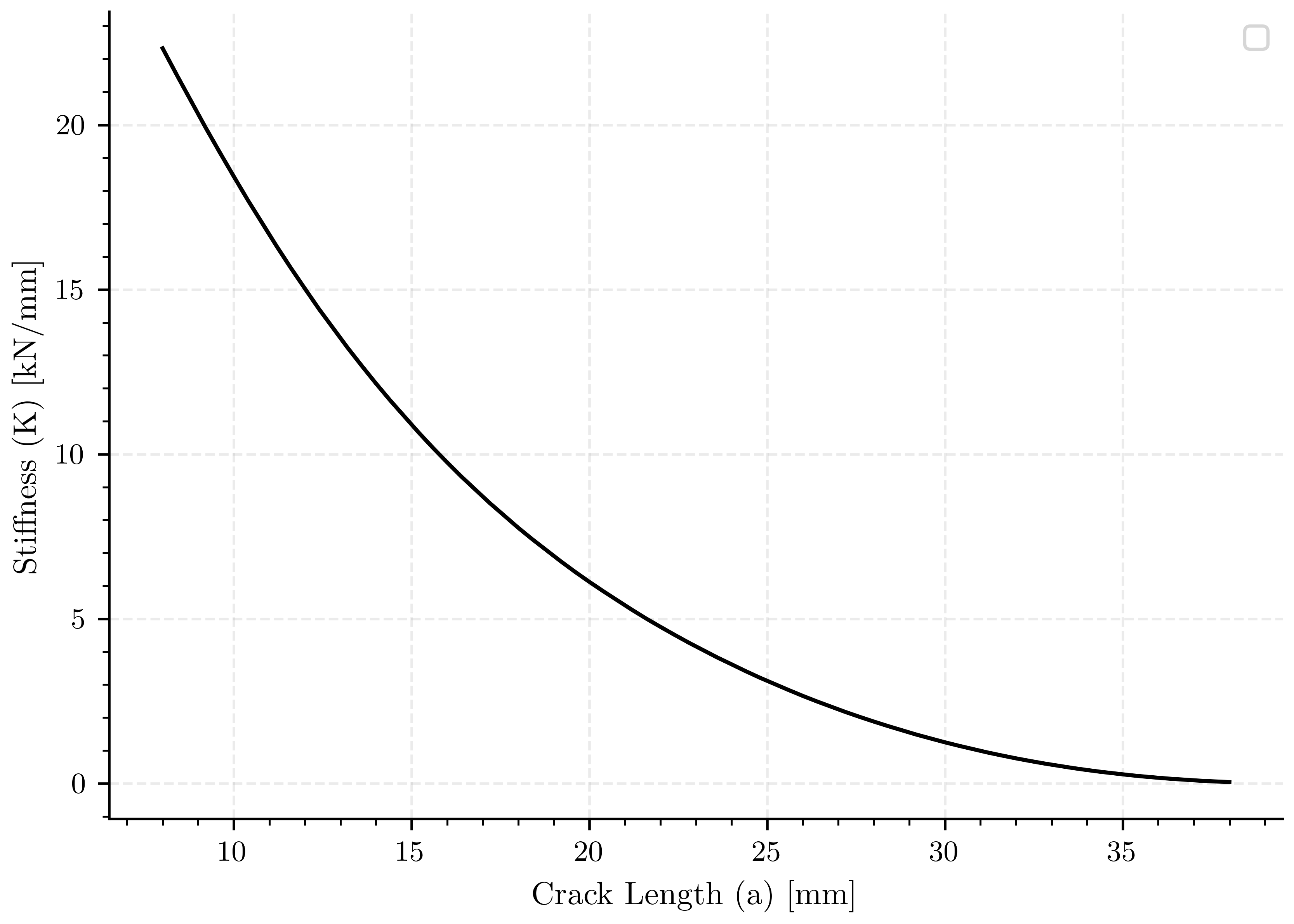
Crack length vs stiffness#
fig, ax0 = plt.subplots()

ax0.plot(a_saved, stiffness_complete_model, 'k-')

ax0.set_xlabel(pcfg.crack_length_label)
ax0.set_ylabel(pcfg.stiffness_label)
ax0.legend()

plt.show()
/home/docs/checkouts/readthedocs.org/user_builds/phasefieldfatigue/checkouts/stable/examples/Elasticity/plot_compact_tension_gmsh.py:320: UserWarning: No artists with labels found to put in legend.  Note that artists whose label start with an underscore are ignored when legend() is called with no argument.
  ax0.legend()
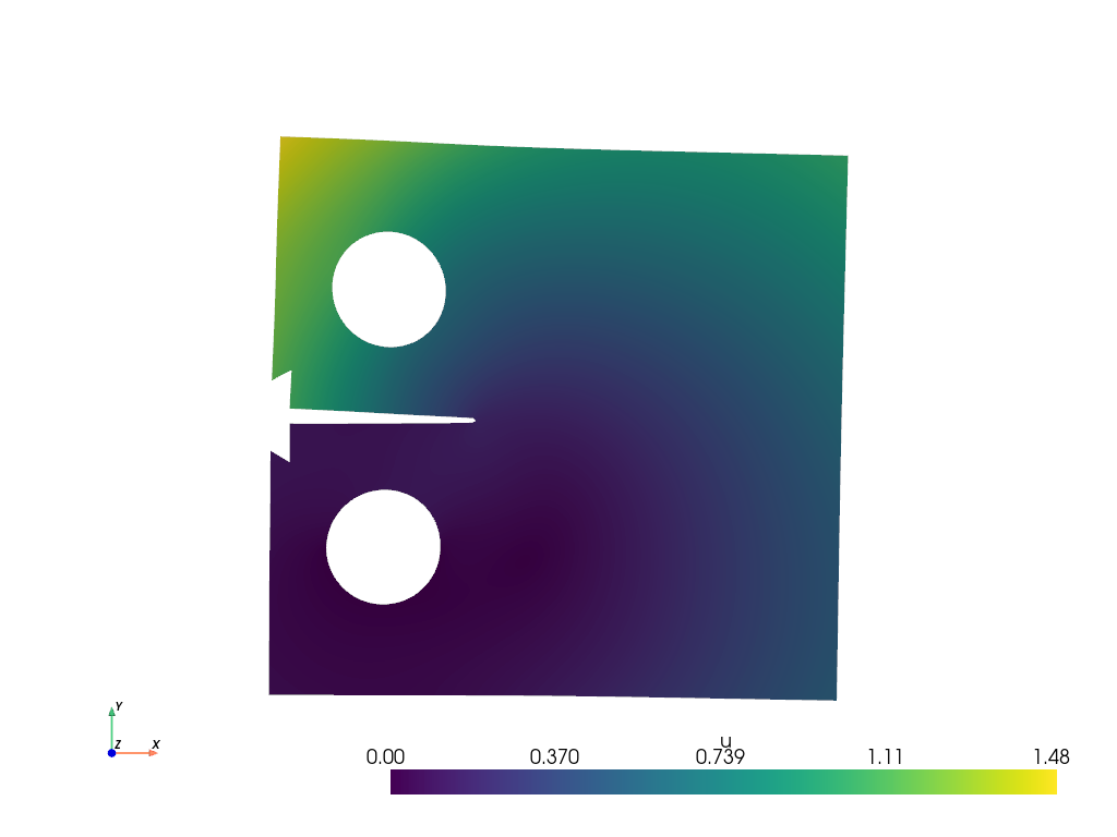
Visualization of Results#
The following section visualizes the mesh and displacement field for two different simulations (indices 20 and 50). The mesh is shown first, followed by the displacement field, which is warped by the displacement vector for better visualization.
pv.start_xvfb()
file_vtu_1 = pv.read(os.path.join(results_folder, "0", "paraview-solutions_vtu", "phasefieldx_p0_000000.vtu"))
file_vtu_2 = pv.read(os.path.join(results_folder, "20", "paraview-solutions_vtu", "phasefieldx_p0_000000.vtu"))
file_vtu_3 = pv.read(os.path.join(results_folder, "45", "paraview-solutions_vtu", "phasefieldx_p0_000000.vtu"))
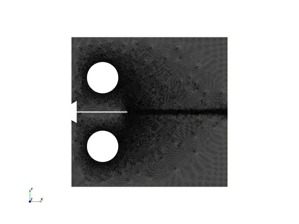
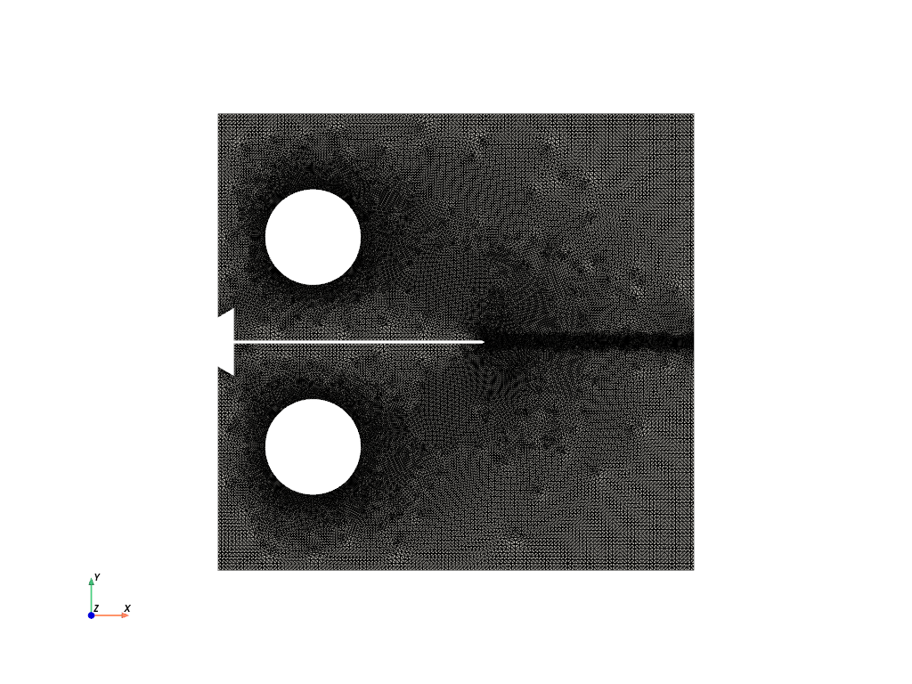
Plot: Mesh#
Display the mesh for the first simulation (index 20).
file_vtu_1.plot(cpos='xy', color='white', show_edges=True)
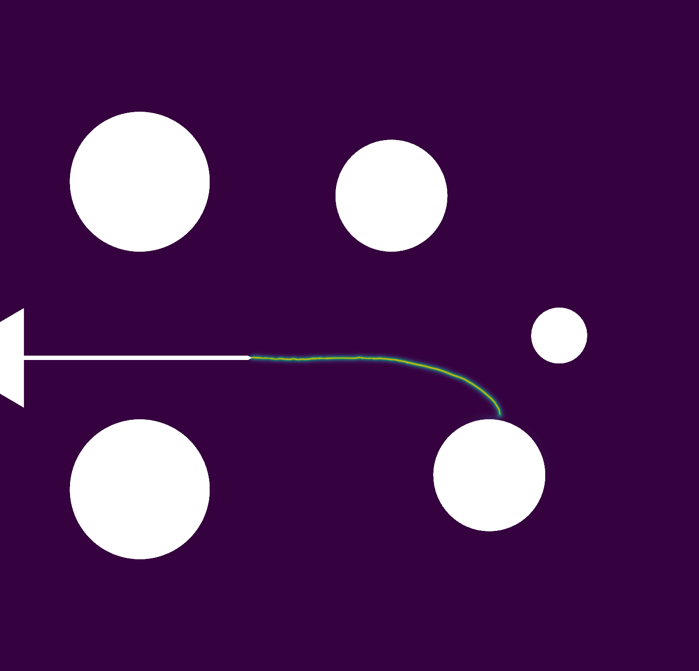
Plot: Displacement (Simulation 20)#
Warp the mesh by the displacement vector for the first simulation and plot the displacement field.
warped_1 = file_vtu_1.warp_by_vector('u', factor=1.0)
warped_1.plot(scalars='u', cpos='xy', show_scalar_bar=True, show_edges=False)
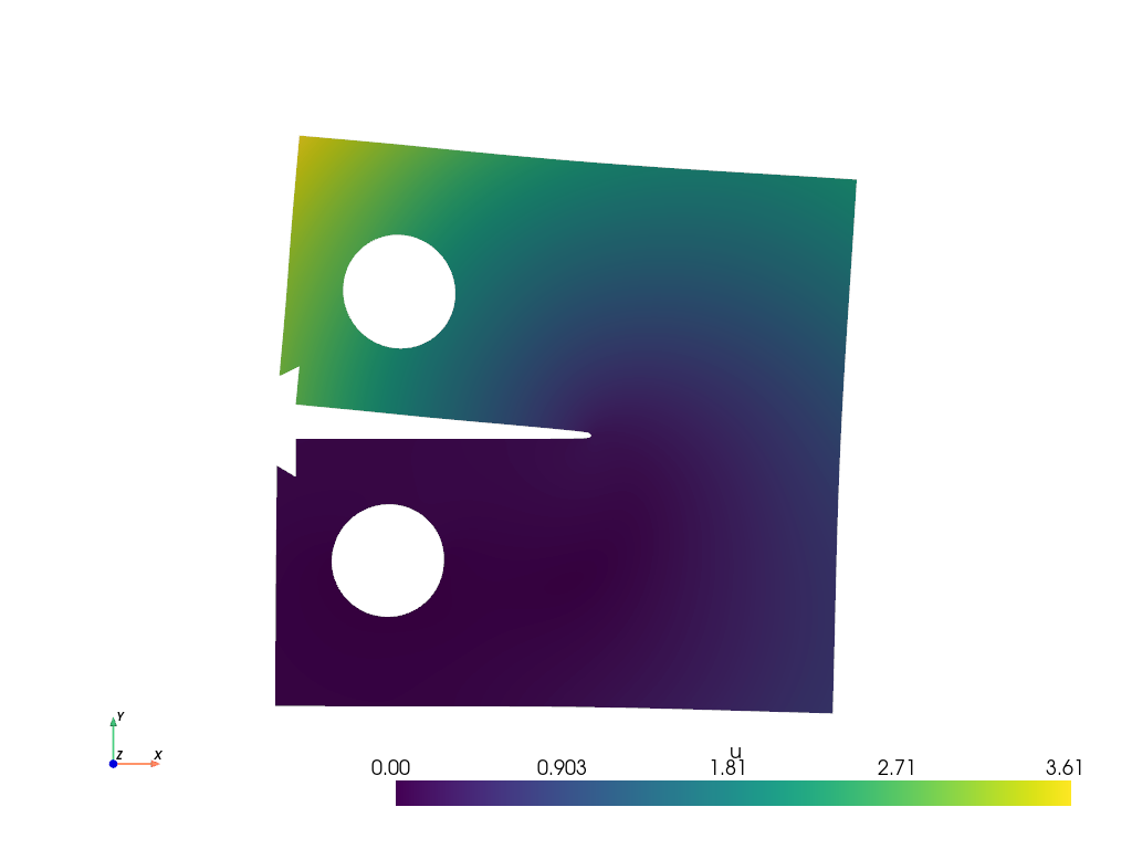
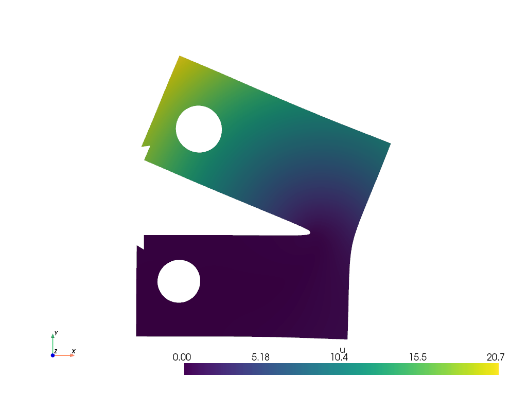
Plot: Displacement (Simulation 50)#
Warp the mesh by the displacement vector for the second simulation and plot the displacement field.
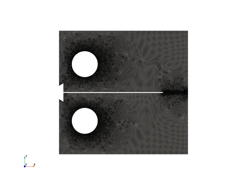
file_vtu_2.plot(cpos='xy', color='white', show_edges=True)
warped_2 = file_vtu_2.warp_by_vector('u', factor=1.0)
warped_2.plot(scalars='u', cpos='xy', show_scalar_bar=True, show_edges=False)
Plot: Displacement (Simulation 50)#
Warp the mesh by the displacement vector for the second simulation and plot the displacement field.
file_vtu_3.plot(cpos='xy', color='white', show_edges=True)
warped_3 = file_vtu_3.warp_by_vector('u', factor=1.0)
warped_3.plot(scalars='u', cpos='xy', show_scalar_bar=True, show_edges=False)

plt.show()


# plotter = pv.Plotter(off_screen=True)  # Use off_screen=True for saving
# plotter.add_mesh(file_vtu_1, show_edges=True)  # show_edges=True to display mesh edges
# plotter.view_xy()
# # plotter.remove_scalar_bar()  # Remove color bar if you don't want it
# plotter.set_background('white')  # Set background color
# bounds = file_vtu_1.bounds  # [xmin, xmax, ymin, ymax, zmin, zmax]
# plotter.camera.tight(padding=0.0)  # No padding at all
# plotter.camera.clipping_range = (0.1, 1000.0)
# plotter.window_size = (500*2, 480*2)  # Adjust width/height ratio as needed
# plotter.screenshot(os.path.join(results_folder,'paraview_mesh_1.png'),
#                   transparent_background=False,
#                   return_img=False)
# plotter.close()


# plotter = pv.Plotter(off_screen=True)  # Use off_screen=True for saving
# plotter.add_mesh(file_vtu_2, show_edges=True)  # show_edges=True to display mesh edges
# plotter.view_xy()
# # plotter.remove_scalar_bar()  # Remove color bar if you don't want it
# plotter.set_background('white')  # Set background color
# bounds = file_vtu_2.bounds  # [xmin, xmax, ymin, ymax, zmin, zmax]
# plotter.camera.tight(padding=0.0)  # No padding at all
# plotter.camera.clipping_range = (0.1, 1000.0)
# plotter.window_size = (500*2, 480*2)  # Adjust width/height ratio as needed
# plotter.screenshot(os.path.join(results_folder,'paraview_mesh_2.png'),
#                   transparent_background=False,
#                   return_img=False)
# plotter.close()


# # Create a PyVista plotter
# plotter = pv.Plotter(off_screen=True)  # Use off_screen=True for saving

# # Extract the surface of the mesh to ensure only 2D elements are shown
# surface_mesh = file_vtu_3.extract_surface()

# # Add the surface mesh as a solid white surface
# plotter.add_mesh(surface_mesh, color='white', show_edges=False)

# # Add the original quad cell edges as black lines
# plotter.add_mesh(surface_mesh, style='wireframe', color='black', line_width=1)

# # Set the view and background
# plotter.view_xy()
# plotter.set_background('white')  # Set background color
# plotter.camera.tight(padding=0.0)  # No padding at all
# plotter.camera.clipping_range = (0.1, 1000.0)

# # Set the window size and save the screenshot
# plotter.window_size = (500 * 2, 480 * 2)  # Adjust width/height ratio as needed
# plotter.screenshot(os.path.join(results_folder, 'paraview_mesh_3.png'),
#                    transparent_background=False,
#                    return_img=False)
# plotter.close()
Total running time of the script: (0 minutes 10.411 seconds)