Examples#
This directory contains the examples supporting the article, demonstrating various approaches to analyzing crack behavior and material fatigue. The analyses are structured into three main types:
Theoretical LEFM Solutions: Analytical solutions derived from Linear Elastic Fracture Mechanics (LEFM) provide a theoretical baseline for comparison.
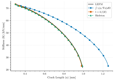
Elasticity Simulations: Numerical analyses are performed on meshes with predefined cracks to calculate the specimen’s compliance and stiffness as a function of crack length.
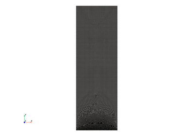
Phase-Field Simulations: The proposed phase-field models are used to simulate crack propagation without requiring predefined crack paths.
The examples are organized into the following directories:
LEFM Analysis: Presents the theoretical analysis based on LEFM. LEFM: Theoretical Analysis and Benchmarks
Elasticity Simulations: Contains elasticity simulations with imposed cracks. FEM: Elasticity Models
Phase-Field Simulations: Includes simulations for three different specimen geometries:
Three-point bending Phase-field: Three Point
Center-cracked specimen Phase-field: Central cracked specimen
Compact specimen Phase-field: Compact specimen
Papers Data: Provides data from published papers for comparison purposes. Papers data
Comparison: Combines results from the different methods for direct comparison.
Central cracked specimen Comparison: Central cracked
Compact specimen Comparison: Compact Specimen
Three-point bending Comparison: Three-Point Bending Test
GmshGeoFiles: Contains the geometry files and instructions for generating the meshes used in the simulations. Gmsh Geometry Files for Meshing
Each Comparison directory corresponds to a validation or results section in the paper, ensuring that the presented graphs align with the discussed findings.
LEFM: Theoretical Analysis and Benchmarks#
This section presents the theoretical analysis based on Linear Elastic Fracture Mechanics (LEFM) for different specimens, including:
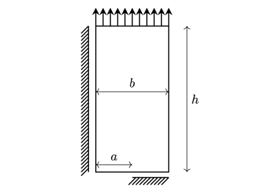
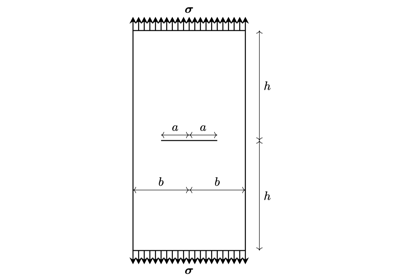
The center-cracked notched tension test.
The three-point bending test.
The ASTM standard test.
These examples are selected because the crack propagation path and geometric factors are well-established, allowing for analytical solutions. This makes it possible to derive theoretical results for evaluating and comparing the proposed framework. Additionally, numerical solutions are obtained by imposing the crack in the mesh and performing simulations for various crack lengths.
The LEFM results presented here form the foundation for validating the phase-field approach. By comparing the analytical solutions derived from LEFM with numerical results, this section demonstrates the consistency and accuracy of the proposed methodology. These examples provide a benchmark for understanding the behavior of fracture mechanics under well-defined conditions.


Compact Tension Specimen: Fracture and Fatigue Analysis
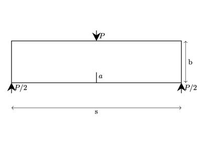
Three-Point Bending Specimen: Fracture and Fatigue Analysis
FEM: Elasticity Models#
This section presents a set of finite element simulations based on linear elastic fracture mechanics (LEFM). The examples include:
Center-cracked tension tests (analyzed under both displacement-controlled and force-controlled loading)
Compact tension specimen (analyzed under force-controlled loading)
For these geometries, the crack path and associated geometry factors are well-established, allowing direct comparison between analytical solutions and numerical results. By explicitly modeling cracks in the mesh and simulating various crack lengths, the computed compliance can be quantitatively compared to LEFM predictions.
Further details on the elasticity model and solver implementation are available in the PhaseFieldX documentation and the PhaseFieldX library.

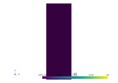
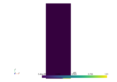
Phase-field: Three Point#
This section presents the simulations for the classical three-point bending test, utilizing both the variational and non-variational phase-field approaches. Identical material parameters, mesh resolution, and boundary conditions are used to ensure a consistent and fair comparison.
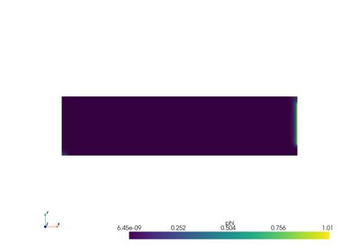
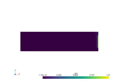
Phase-field: Central cracked specimen#
This section presents six simulations, each considering a quarter of the geometry due to the double symmetry of the central crack tension test specimen. The simulations analyze two different length scales and various initial crack lengths imposed in the mesh. These simulations correspond to the cases shown in the accompanying table. The first column refers to the initial crack length imposed in the mesh through the boundary conditions, and the second and third columns refer to the different length scale parameters considered.
\(a_0\) |
\(l_1 = 0.025\) mm |
\(l_2 = 0.0025\) mm |
|---|---|---|
\(0.3\) mm |
||
\(0.5\) mm |
||
\(0.7\) mm |
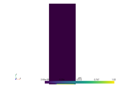
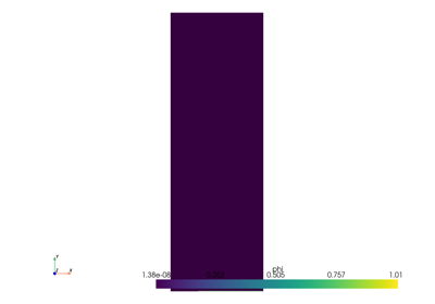


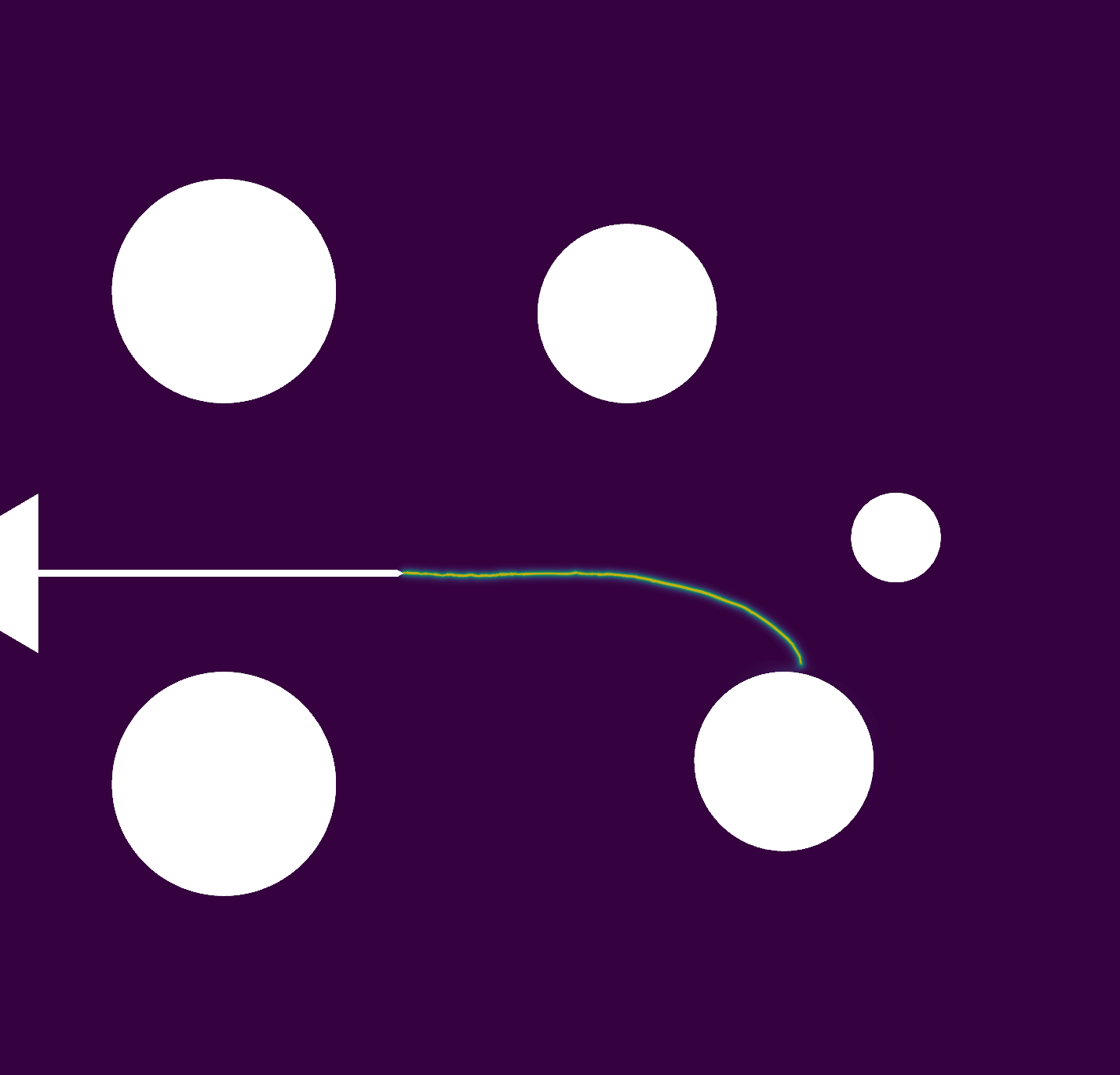
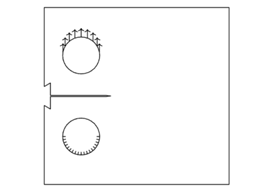
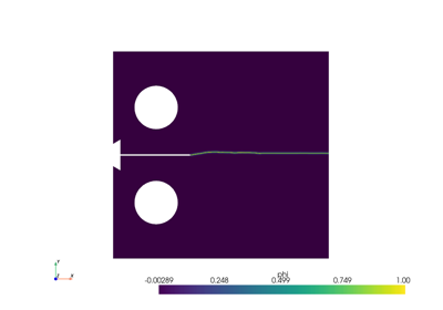
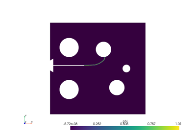
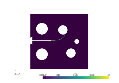
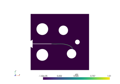
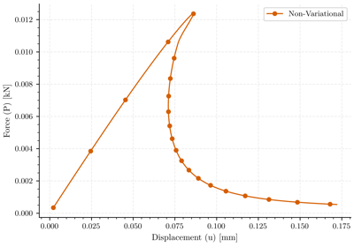
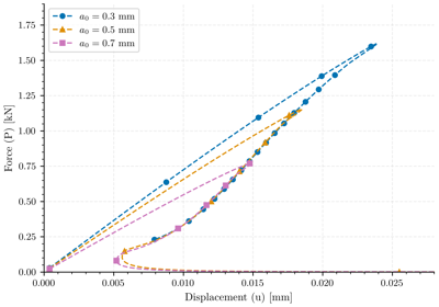
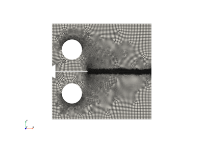
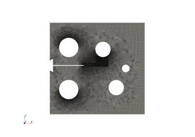
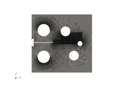
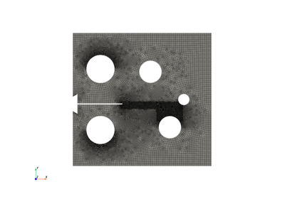
Phase-field: Compact specimen#
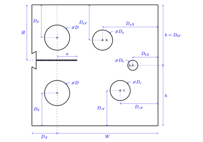
In this section, the specimens described in Wagner[1] are simulated using the phase-field model proposed in the referenced work.
Four simulations are conducted, each with distinct configurations:
Specimen |
H (Crack Position) |
Holes Considered |
|---|---|---|
\(H = 0.60 W = 24.0\) mm |
No holes |
|
\(H = 0.56 W = 22.4\) mm |
With holes |
|
\(H = 0.58 W = 23.2\) mm |
With holes |
|
\(H = 0.64 W = 25.6\) mm |
With holes |
Comparison: Three-Point Bending Test#
This section presents two examples comparing the variational and non-variational solvers. To demonstrate their equivalence, as explained in the referenced paper, both examples use an identical setup, including the same mesh, materials, and boundary conditions. The only difference is the solver used in each case.
Comparison: Central cracked#
Several aspects must be considered when working with phase-field models, such as the length scale parameter, mesh size, and energy split method. Additionally, it is important to account for the crack area and how it is treated in the simulation. In this section, we analyze the influence of these parameters on the results.
Length Scale Parameter Study for Phase-Field Fracture
Comparison: Compact Specimen#


Gmsh Geometry Files for Meshing#
This directory contains the Gmsh .geo files used to generate the finite element meshes for all simulations presented in the paper. These geometry scripts are essential for reproducing the exact specimen models analyzed in the study.
For detailed information on Gmsh and its scripting language, please refer to the official Gmsh documentation.
To generate a 2D mesh from a .geo file, you can use the following command in your terminal:
gmsh your_file.geo -2 -o your_mesh.msh
Command Breakdown:
gmsh your_file.geo: Runs Gmsh on your specified geometry file.-2: Instructs Gmsh to generate a 2D mesh.-o your_mesh.msh: Specifies the output file name for the generated mesh.
This command will create a .msh file that can be used in the finite element simulations.
Papers data#
This section presents data derived from Wagner[1], which were used for comparison purposes.
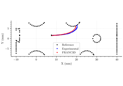
Visualization of Experimental and Simulation Data from Wagner’s PhD Thesis
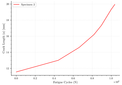
Visualization of Experimental and Simulation Data from Wagner