Note

Go to the end to download the full example code.

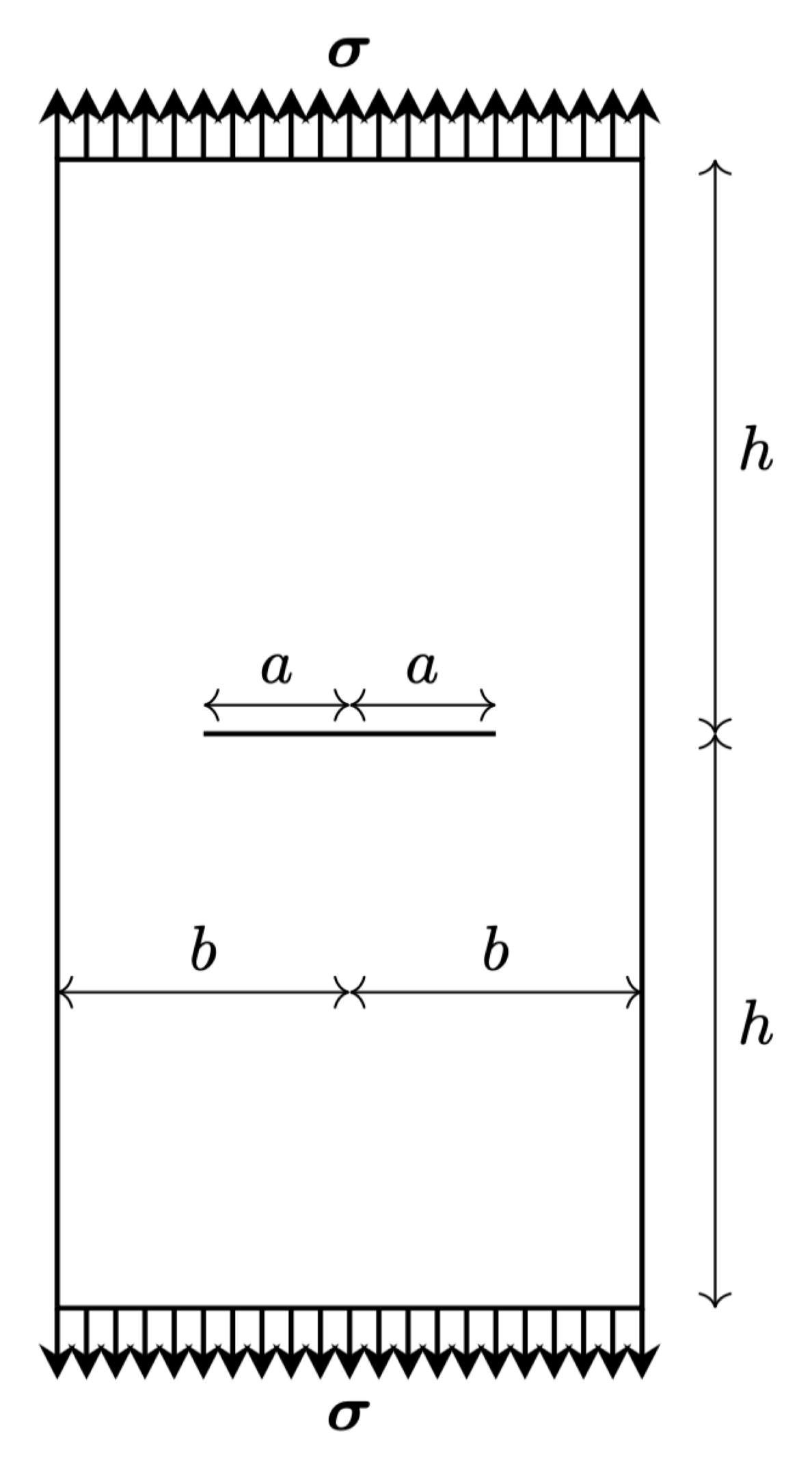
Central cracked specimen#

This script generates a plot comparing the stiffness of a centrally cracked specimen as a function of crack length. The results include four different approaches:

Displacement-Controlled Loading: Stiffness values obtained under displacement-controlled conditions. The displacement-controlled simulation results are generated in the script Displacement Controlled Center Cracked Specimen.
Force-Controlled Loading: Stiffness values obtained under force-controlled conditions. The force-controlled simulation results are generated in the script Force Controlled Center Cracked Specimen.
LEFM Theory: Theoretical predictions based on Linear Elastic Fracture Mechanics (LEFM). The LEFM results are generated in the script LEFM: Center-Cracked Specimen.

Finally, the script also includes results from a phase-field simulation of a centrally cracked specimen.

The purpose of this script is to visualize and compare the stiffness behavior of the specimen under different loading conditions and theoretical predictions.

Import necessary libraries#

import numpy as np
import pandas as pd
import matplotlib.pyplot as plt
import matplotlib.image as mpimg
import os
import shutil
import pandas as pd
import sys
sys.path.insert(0, os.path.abspath('../../'))
plt.style.use('../../graph.mplstyle')
import plot_config as pcfg

img = mpimg.imread('images/central_cracked.png')  # or .jpg, .tif, etc.
plt.imshow(img)
plt.axis('off')

results_folder = "results_central_cracked"
if os.path.exists(results_folder):
    shutil.rmtree(results_folder)
os.makedirs(results_folder, exist_ok=True)

Parameters definition#

Define material and specimen parameters

E  = 210  # Young's modulus (kN/mm^2)
nu = 0.3  # Poisson's ratio (-)
Gc = 0.0027  # Critical strain energy release rate (kN/mm)
Cparis = 1.33e-10  # Paris' Law constant C
m = 3.5          # Paris' Law exponent m
Ep = E / (1.0 - nu**2) # Plane strain modulus (kN/mm^2)

# %
# Specimen geometry
B = 1.0  # Specimen thickness (mm)

Load the results#

%% From FEM elastic displacement controlled simulation Displacement Controlled Center Cracked Specimen

displacement_control = pd.read_csv("../Elasticity/results_center_cracked_displacement_control/results.elasticity", delimiter="\t", comment="#", header=0)
LABEL_DISPLACEMENT = r"Elasticity: Displacement-controlled"
LABEL_FORCE = r"Elasticity: Force-controlled"
LABEL_LEFM = r"LEFM (Analytical)"

# Colors from plot_config.py
COLOR_DISPLACEMENT = pcfg.color_blue
COLOR_FORCE = pcfg.color_orangered
COLOR_LEFM = pcfg.color_black
COLOR_PHASEFIELD = pcfg.color_green
a_disp = displacement_control["crack_length"]
k_disp = displacement_control["stiffness"]
c_disp = 1/k_disp
dCda_disp = np.gradient(c_disp, a_disp)
pc_disp = np.sqrt(2*B*Gc/(0.5*dCda_disp))

From FEM elastic force controlled simulation Force Controlled Center Cracked Specimen

force_control = pd.read_csv("../Elasticity/results_center_cracked_force_control/results.elasticity", delimiter="\t", comment="#", header=0)

a_forc = force_control["crack_length"]
k_forc = force_control["stiffness"]
c_forc = 1/k_forc
dCda_forc = np.gradient(c_forc, a_forc)
pc_forc = np.sqrt(2*B*Gc/(0.5*dCda_forc))

From Linear elastic fracture mechanics theory LEFM: Center-Cracked Specimen SCHEME_3 = np.loadtxt(“../LEFM/results_central_cracked/center_cracked.lefm”, delimiter=”t”, skiprows=1)

lefm = pd.read_csv("../LEFM/results_central_cracked/center_cracked.lefm", delimiter="\t", comment="#", header=0)
LABEL_LEFM = r"LEFM (Analytical)"
a_lefm = lefm["a"]
k_lefm = 1/lefm["C"]
c_lefm = lefm["C"]
pc_lefm = lefm["Pc"]

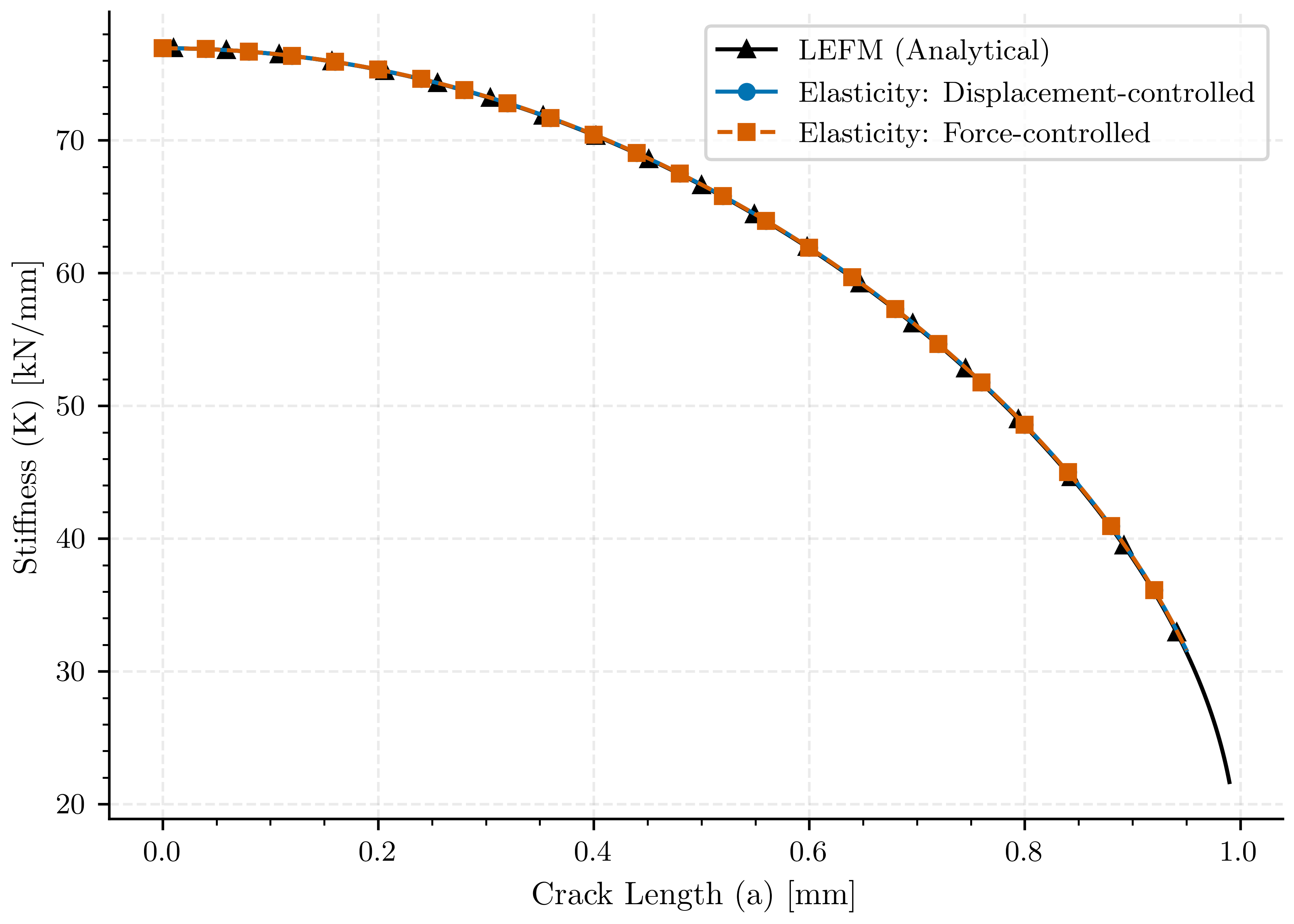
Crack length vs stiffness#

The stiffness as function of crack length is plotted for the three methods.

# Proportional marker spacing
markevery_disp = max(1, len(a_disp)//20)
markevery_forc = max(1, len(a_forc)//20)
markevery_lefm = max(1, len(a_lefm)//20)

fig, ax0 = plt.subplots()
ax0.plot(a_lefm, k_lefm, color=COLOR_LEFM, linestyle='-', marker='^', label=LABEL_LEFM, markevery=markevery_lefm)
ax0.plot(a_disp, k_disp, color=COLOR_DISPLACEMENT, linestyle='-', marker='o', label=LABEL_DISPLACEMENT, markevery=markevery_disp)
ax0.plot(a_forc, k_forc, color=COLOR_FORCE, linestyle='--', marker='s', label=LABEL_FORCE, markevery=markevery_forc)


# Enhance plot aesthetics
ax0.set_xlabel(pcfg.crack_length_label)
ax0.set_ylabel(pcfg.stiffness_label)
ax0.legend()

# Save the figure
plt.savefig(os.path.join(results_folder, "stiffness_vs_crack_length"))

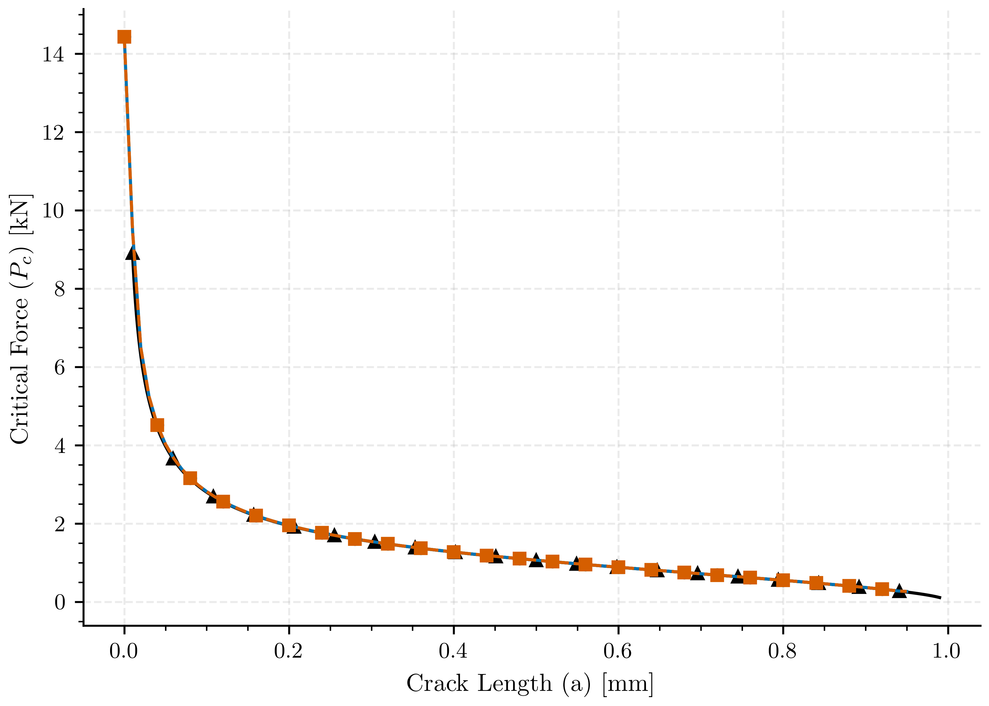
Crack length vs stiffness#

The stiffness as function of crack length is plotted for the three methods.

fig, ax0 = plt.subplots()

ax0.plot(a_lefm, pc_lefm, color=COLOR_LEFM, linestyle='-', marker='^', label=LABEL_LEFM, markevery=markevery_lefm)
ax0.plot(a_disp, pc_disp, color=COLOR_DISPLACEMENT, linestyle='-', marker='o', label=LABEL_DISPLACEMENT, markevery=markevery_disp)
ax0.plot(a_forc, pc_forc, color=COLOR_FORCE, linestyle='--', marker='s', label=LABEL_FORCE, markevery=markevery_forc)


# Enhance plot aesthetics
ax0.set_xlabel(pcfg.crack_length_label)
ax0.set_ylabel(pcfg.critical_force_label)
# ax0.legend()

# Save the figure
plt.savefig(os.path.join(results_folder, "critical_force_vs_crack_length"))

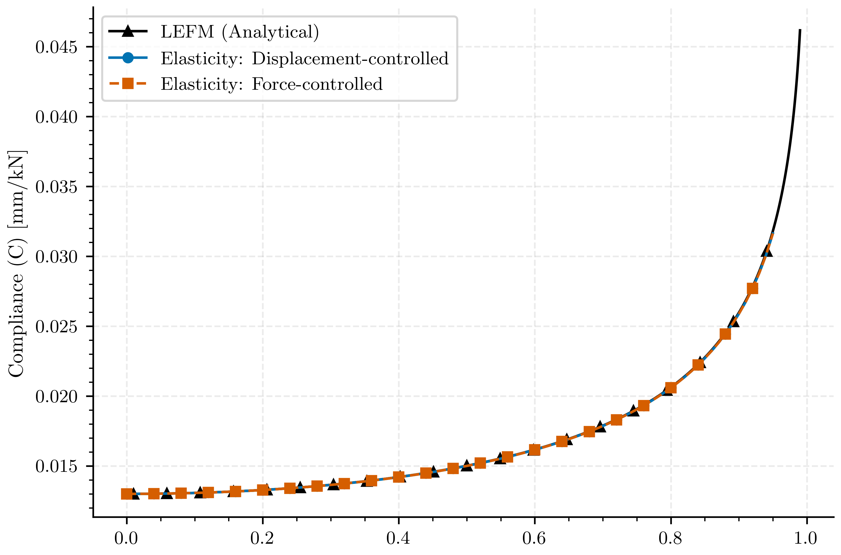
Crack length vs compliance#

The compliance as function of crack length is plotted for the three methods:

fig, ax1 = plt.subplots()
ax1.plot(a_lefm, c_lefm, color=COLOR_LEFM, linestyle='-', marker='^', label=LABEL_LEFM, markevery=markevery_lefm)

ax1.plot(a_disp, c_disp, color=COLOR_DISPLACEMENT, linestyle='-', marker='o', label=LABEL_DISPLACEMENT, markevery=markevery_disp)
ax1.plot(a_forc, c_forc, color=COLOR_FORCE, linestyle='--', marker='s', label=LABEL_FORCE, markevery=markevery_forc)

# Enhance plot aesthetics
ax0.set_xlabel(pcfg.crack_length_label)
ax1.set_ylabel(pcfg.compliance_label)
ax1.legend()

# Save the figure
plt.savefig(os.path.join(results_folder,"compliance_vs_crack_length") )

Fatigue#

Once the compliance curves are obtained, it is possible to calculate the fatigue lives from the compliance respect the crack area for the different methods. In this case the fatigue analysis is performed for a crack that goes from an initial crack length value_1 to a final crack length value_2.

a0_fatigue = 0.4 # Initial crack length [mm]
af_fatigue = 0.9 # Final crack length [mm]

To perform the fatigue analysis in that range, will be needed to tlice the arrays to obtain the values of the compliance and crack area in that range.

def slice_array_by_values(a, value_1, value_2):
    """
    Returns a slice of the array `a` between the indices of the nearest values to `value_1` and `value_2`.

    Parameters:
    a (numpy.ndarray): The input array.
    value_1 (float): The first value to find in the array.
    value_2 (float): The second value to find in the array.

    Returns:
    numpy.ndarray: A new array sliced between the indices of the nearest values to `value_1` and `value_2`.
    """
    # Find the indices of the nearest values
    index_1 = (np.abs(a - value_1)).argmin()
    index_2 = (np.abs(a - value_2)).argmin()

    # Ensure index_1 is less than index_2
    if index_1 > index_2:
        index_1, index_2 = index_2, index_1

    # Return the sliced array
    return index_1, index_2 + 1

Slice the arrays to obtain the fatigue region

i_o_1, i_f_1 = slice_array_by_values(a_disp, a0_fatigue, af_fatigue)
i_o_2, i_f_2 = slice_array_by_values(a_forc, a0_fatigue, af_fatigue)
i_o_3, i_f_3 = slice_array_by_values(a_lefm, a0_fatigue, af_fatigue)

Extract the fatigue regions

a_fatigue_disp, c_fatigue_disp = a_disp[i_o_1:i_f_1], c_disp[i_o_1:i_f_1]
a_fatigue_forc, c_fatigue_forc = a_forc[i_o_2:i_f_2], c_forc[i_o_2:i_f_2]
a_fatigue_lefm, c_fatigue_lefm = a_lefm[i_o_3:i_f_3], c_lefm[i_o_3:i_f_3]

Then, the derivative of the compliance respect the crack area is calculated for each method.

dCda_fatigue_disp = np.gradient(c_fatigue_disp, a_fatigue_disp)
dCda_fatigue_forc = np.gradient(c_fatigue_forc, a_fatigue_forc)
dCda_fatigue_lefm = np.gradient(c_fatigue_lefm, a_fatigue_lefm)

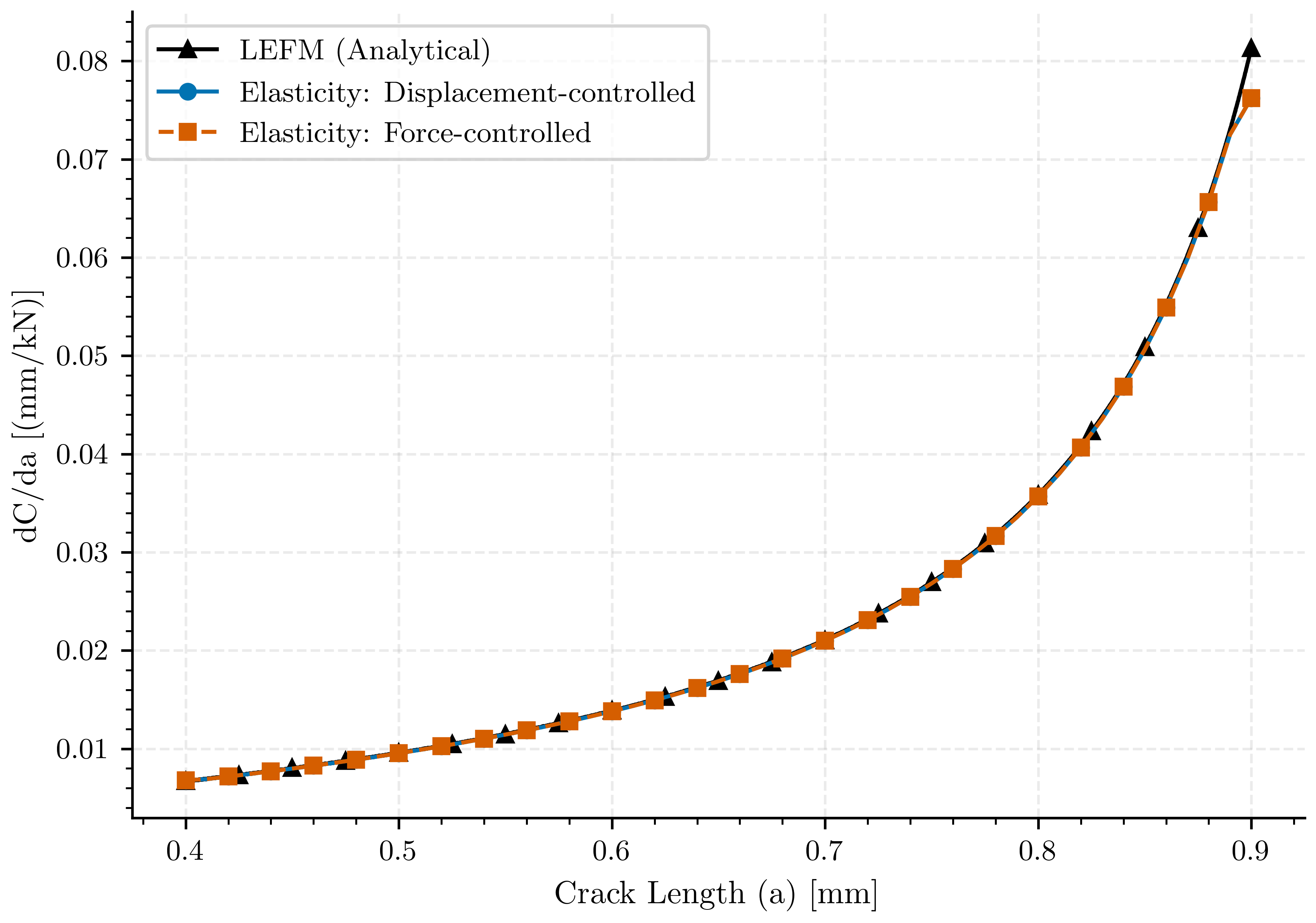
Crack area vs \(dC/da\)#

The derivative of the compliance respect the crack area is plotted for the three methods.

markevery_fatigue_disp = max(1, len(a_fatigue_disp)//20)
markevery_fatigue_forc = max(1, len(a_fatigue_forc)//20)
markevery_fatigue_lefm = max(1, len(a_fatigue_lefm)//20)

fig, ax2 = plt.subplots()
ax2.plot(a_fatigue_lefm, dCda_fatigue_lefm, color=COLOR_LEFM, linestyle='-', marker='^', label=LABEL_LEFM, markevery=markevery_fatigue_lefm)
ax2.plot(a_fatigue_disp, dCda_fatigue_disp, color=COLOR_DISPLACEMENT, linestyle='-', marker='o', label=LABEL_DISPLACEMENT, markevery=markevery_fatigue_disp)
ax2.plot(a_fatigue_forc, dCda_fatigue_forc, color=COLOR_FORCE, linestyle='--', marker='s', label=LABEL_FORCE, markevery=markevery_fatigue_forc)


# Enhance plot aesthetics
ax2.set_xlabel(pcfg.crack_length_label)
ax2.set_ylabel(pcfg.dCda_label)
ax2.legend()

<matplotlib.legend.Legend object at 0x734c5e29ba30>

Once, the derivative of the compliance respect the crack area is calculated, it is possible to calculate the number of cycles to failure using the Paris law. In this case, the Paris law is used in the form: .. math:

N_f = N_i + \frac{1}{C_{Paris} \left(\frac{E_p}{2B}\right)^{m/2} A_P} \int_{a_i}^{a_f} \left(\frac{dC}{da}\right)^{-m/2} da

The initial number of cycles is set to zero, and the Paris law parameters are defined as follows:

AP = 33.0      # Applied cyclic force range (Delta_P) [kN]
Ni = 0         # Initial number of cycles

from scipy.integrate import cumulative_trapezoid, cumulative_simpson

Calculate the number of cycles to failure for each method. The integration is performed using the trapezoidal rule.

Nf_dCda_1 = Ni + 1/(Cparis * (Ep/(2*B))**(m/2) * AP**m)*cumulative_trapezoid(1/(dCda_fatigue_disp)**(m/2), a_fatigue_disp, initial=0)
Nf_dCda_2 = Ni + 1/(Cparis * (Ep/(2*B))**(m/2) * AP**m)*cumulative_trapezoid(1/(dCda_fatigue_forc)**(m/2), a_fatigue_forc, initial=0)
Nf_dCda_3 = Ni + 1/(Cparis * (Ep/(2*B))**(m/2) * AP**m)*cumulative_trapezoid(1/(dCda_fatigue_lefm)**(m/2), a_fatigue_lefm, initial=0)

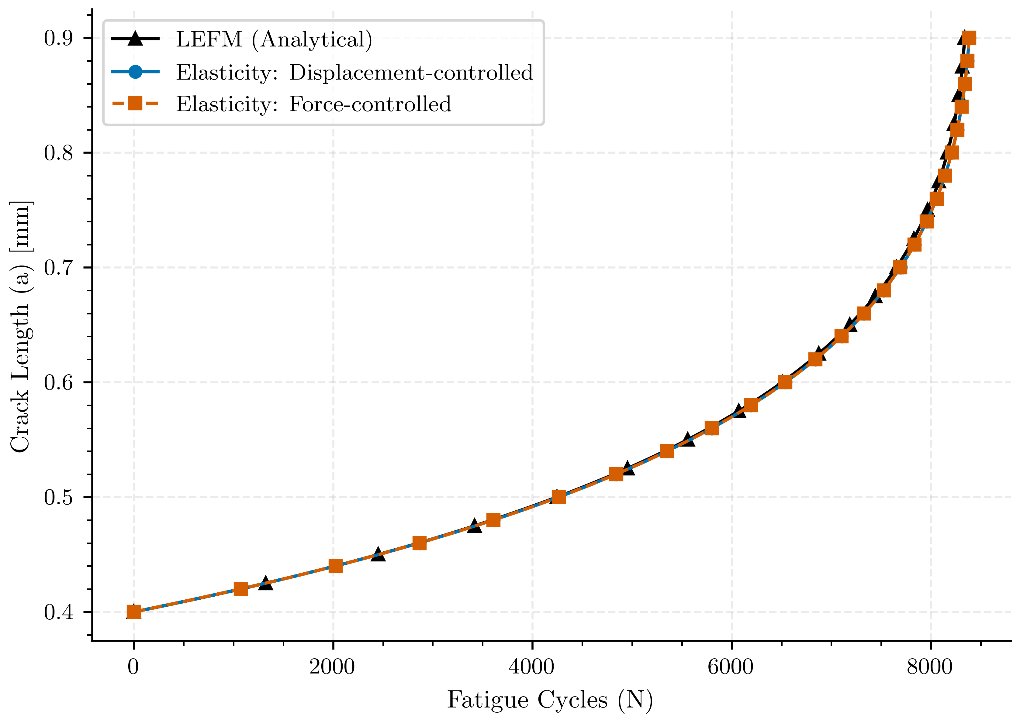
Crack area vs number of cycles#

The number of cycles to failure is calculated from the compliance respect the crack area for the different methods.

fig, ax3 = plt.subplots()
ax3.plot(Nf_dCda_3, a_fatigue_lefm, color=COLOR_LEFM, linestyle='-', marker='^', label=LABEL_LEFM, markevery=markevery_fatigue_lefm)
ax3.plot(Nf_dCda_1, a_fatigue_disp, color=COLOR_DISPLACEMENT, linestyle='-', marker='o', label=LABEL_DISPLACEMENT, markevery=markevery_fatigue_disp)
ax3.plot(Nf_dCda_2, a_fatigue_forc, color=COLOR_FORCE, linestyle='--', marker='s', label=LABEL_FORCE, markevery=markevery_fatigue_forc)


# Enhance plot aesthetics
ax3.set_ylabel(pcfg.crack_length_label)
ax3.set_xlabel(pcfg.cycles_label)
ax3.legend()

plt.savefig(os.path.join(results_folder, "cycles_vs_crack_length"))


# ###############################################################################
# # Fatigue analysis for phase-field method
# # ---------------------------------------
# # For the fatigue analysis of the phase-field method, the derivative of the compliance respect the crack area is calculated from the results of the phase-field simulation.
# import pandas as pd
# # Load the data (skip the first line if it's a comment, otherwise just use header=0)


# file = "../Phase_Field_Central_Craked/results_2_a03_l2/results.pff"
# df = pd.read_csv(file, delim_whitespace=True, comment='/', header=0)

# a_phas = df["gamma"]  # Crack area
# dCda_phas = 2*df["dCda"]

# a_phas_geo = df["gamma_corrected_measure"]  # Crack area
# dCda_phas_geo = 2*df["dCda_corrected_measure"]

# a_phas_Gc = df["gamma_corrected_Gc"]  # Crack area
# dCda_phas_Gc = df["dCda_corrected_Gc"]

# k_phas = 1/df["compliance"]
# c_phas = df["compliance"]

# # dCda_phas = np.gradient(c_phas, a_phas)


# # gamma_corrected_measure dCda_corrected_measure





# ###############################################################################
# # Crack length vs stiffness
# # -------------------------
# # The stiffness as function of crack length is plotted for the three methods.
# fig, ax0 = plt.subplots()

# ax0.plot(a_lefm, pc_lefm, color=COLOR_LEFM, linestyle='-', marker='^', label=LABEL_LEFM, markevery=markevery_lefm)
# ax0.plot(a_phas, np.sqrt(2*2*B*Gc/dCda_phas), linestyle='--')
# ax0.plot(a_phas_Gc, np.sqrt(2*2*B*Gc/dCda_phas_Gc), linestyle='--')
# ax0.plot(a_phas_geo, np.sqrt(2*2*B*Gc/dCda_phas_geo), linestyle='--')


# # Enhance plot aesthetics
# ax0.set_xlabel(pcfg.crack_length_label)
# ax0.set_ylabel(pcfg.critical_force_label)
# # ax0.legend()

# # Save the figure
# plt.savefig(os.path.join(results_folder, "critical_force_vs_crack_length_pff"))



# ###############################################################################
# # Fatigue
# # -------
# # Once the compliance curves are obtained, it is possible to calculate the fatigue lives from the compliance respect the crack area for the different methods.
# # In this case the fatigue analysis is performed for a crack that goes from an initial crack length `value_1` to a final crack length `value_2`.

# def slice_array_by_values(a, value_1, value_2):
#     """
#     Returns a slice of the array `a` between the indices of the nearest values to `value_1` and `value_2`.

#     Parameters:
#     a (numpy.ndarray): The input array.
#     value_1 (float): The first value to find in the array.
#     value_2 (float): The second value to find in the array.

#     Returns:
#     numpy.ndarray: A new array sliced between the indices of the nearest values to `value_1` and `value_2`.
#     """
#     # Find the indices of the nearest values
#     index_1 = (np.abs(a - value_1)).argmin()
#     index_2 = (np.abs(a - value_2)).argmin()

#     # Ensure index_1 is less than index_2
#     if index_1 > index_2:
#         index_1, index_2 = index_2, index_1

#     # Return the sliced array
#     return index_1, index_2 + 1

# # %%
# # Slice the arrays to obtain the fatigue region
# a0 = 0.4
# i_o_1, i_f_1 = slice_array_by_values(a_phas_geo,  a0, 0.9)
# a_fatigue_1, c_fatigue_1 = a_phas_geo[i_o_1:i_f_1], a_phas_geo[i_o_1:i_f_1]
# dCda_fatigue_1 = dCda_phas_geo[i_o_1:i_f_1]



# ###############################################################################
# # Crack length vs stiffness
# # -------------------------

# markevery_phas = max(1, len(a_phas_geo)//20)
# fig, ax4 = plt.subplots()
# ax4.plot(a_lefm, k_lefm, color=COLOR_LEFM, linestyle='--', marker='^', label=LABEL_LEFM, markevery=markevery_lefm)
# ax4.plot(a_disp, k_disp, color=COLOR_DISPLACEMENT, linestyle='-', marker='o', label=LABEL_DISPLACEMENT, markevery=markevery_disp)
# ax4.plot(a_forc, k_forc, color=COLOR_FORCE, linestyle='--', marker='s', label=LABEL_FORCE, markevery=markevery_forc)

# ax4.plot(a_phas_geo, k_phas, color=COLOR_PHASEFIELD, linestyle='--', marker='D', label=r"Phase-field", markevery=markevery_phas)
# ax4.plot(a_phas_Gc, k_phas, color=COLOR_PHASEFIELD, linestyle='--', marker='D', label=r"Phase-field", markevery=markevery_phas)


# ax4.plot(df["gamma"], k_phas, color='b', linestyle='-', marker='v', label=r"gamma", markevery=markevery_phas)
# ax4.plot(df["gamma_corrected_Gc"], k_phas, color='b', linestyle='--', marker='x', label=r"gamma correction", markevery=markevery_phas)
# ax4.plot(df["double_gradphi"], k_phas, color='y', linestyle='-', marker='P', label=r"double gradphi", markevery=markevery_phas)

# # Enhance plot aesthetics
# ax4.set_xlabel(pcfg.crack_length_label)
# ax4.set_ylabel(pcfg.stiffness_label)
# ax4.legend()
# plt.savefig(os.path.join(results_folder,"compare_stiffness_phase_field"))


# # %%
# # Extract the fatigue regions
# i_o_4, i_f_4 = slice_array_by_values(a_phas_geo, a0_fatigue, af_fatigue)
# a_fatigue_phas, c_fatigue_phas = a_phas_geo[i_o_4:i_f_4], c_phas[i_o_4:i_f_4]
# dCda_fatigue_phas = dCda_phas_geo[i_o_4:i_f_4]

# i_o_1, i_f_1 = slice_array_by_values(a_phas_Gc,  a0, 0.9)
# a_fatigue_gc, c_fatigue_gc = a_phas_Gc[i_o_1:i_f_1], c_phas[i_o_1:i_f_1]
# dCda_fatigue_gc = dCda_phas_Gc[i_o_1:i_f_1]


# Nf_dCda_4 = Ni + 1/(Cparis * (Ep/(2*B))**(m/2) * AP**m)*cumulative_trapezoid(1/(dCda_fatigue_phas)**(m/2), a_fatigue_phas, initial=0)
# Nf_dCda_gc = Ni + 1/(Cparis * (Ep/(2*B))**(m/2) * AP**m)*cumulative_trapezoid(1/(dCda_fatigue_gc)**(m/2), a_fatigue_gc, initial=0)


# ###############################################################################
# # Crack length vs stiffness
# # -------------------------

# fig, ax4 = plt.subplots()
# ax4.plot(a_fatigue_lefm, dCda_fatigue_lefm, color=COLOR_LEFM, linestyle='-', marker='^', label=LABEL_LEFM, markevery=markevery_fatigue_lefm)

# ax4.plot(a_fatigue_disp, dCda_fatigue_disp, color=COLOR_DISPLACEMENT, linestyle='-', marker='o', label=LABEL_DISPLACEMENT, markevery=markevery_fatigue_disp)
# ax4.plot(a_fatigue_forc, dCda_fatigue_forc, color=COLOR_FORCE, linestyle='--', marker='s', label=LABEL_FORCE, markevery=markevery_fatigue_forc)

# ax4.plot(a_fatigue_phas, dCda_fatigue_phas, color=COLOR_PHASEFIELD, linestyle='--', marker='D', label=r"Phase-field", markevery=markevery_phas)
# ax4.plot(a_fatigue_gc, dCda_fatigue_gc, color=COLOR_PHASEFIELD, linestyle='--', marker='D', label=r"Phase-field Gc", markevery=markevery_phas)

# # Enhance plot aesthetics
# ax4.set_xlabel(pcfg.crack_length_label)
# ax4.set_ylabel(pcfg.dCda_label)
# ax4.legend()
# plt.savefig(os.path.join(results_folder,"compare_dCda_phase_field"))

Crack length vs number of cycles#

# fig, ax5 = plt.subplots()
# ax5.plot(Nf_dCda_3, a_fatigue_lefm, color=COLOR_LEFM, linestyle='-', marker='^', label=LABEL_LEFM, markevery=markevery_fatigue_lefm)

# ax5.plot(Nf_dCda_2, a_fatigue_forc, color=COLOR_FORCE, linestyle='--', marker='s', label=LABEL_FORCE, markevery=markevery_fatigue_forc)

# ax5.plot(Nf_dCda_4, a_fatigue_phas, color=COLOR_PHASEFIELD, linestyle='--', marker='D', label=r"Phase-field", markevery=markevery_phas)

# ax5.plot(Nf_dCda_gc, a_fatigue_gc, linestyle='--', marker='D', label=r"Phase-field Gc", markevery=markevery_phas)


# # Enhance plot aesthetics
# ax5.set_ylabel(pcfg.crack_length_label)
# ax5.set_xlabel(pcfg.cycles_label)
# ax5.legend()
# plt.savefig(os.path.join(results_folder, "compare_paris_law_phase_field"))

plt.show()

Total running time of the script: (0 minutes 4.872 seconds)

Gallery generated by Sphinx-Gallery