Displacement Controlled Center Cracked Specimen

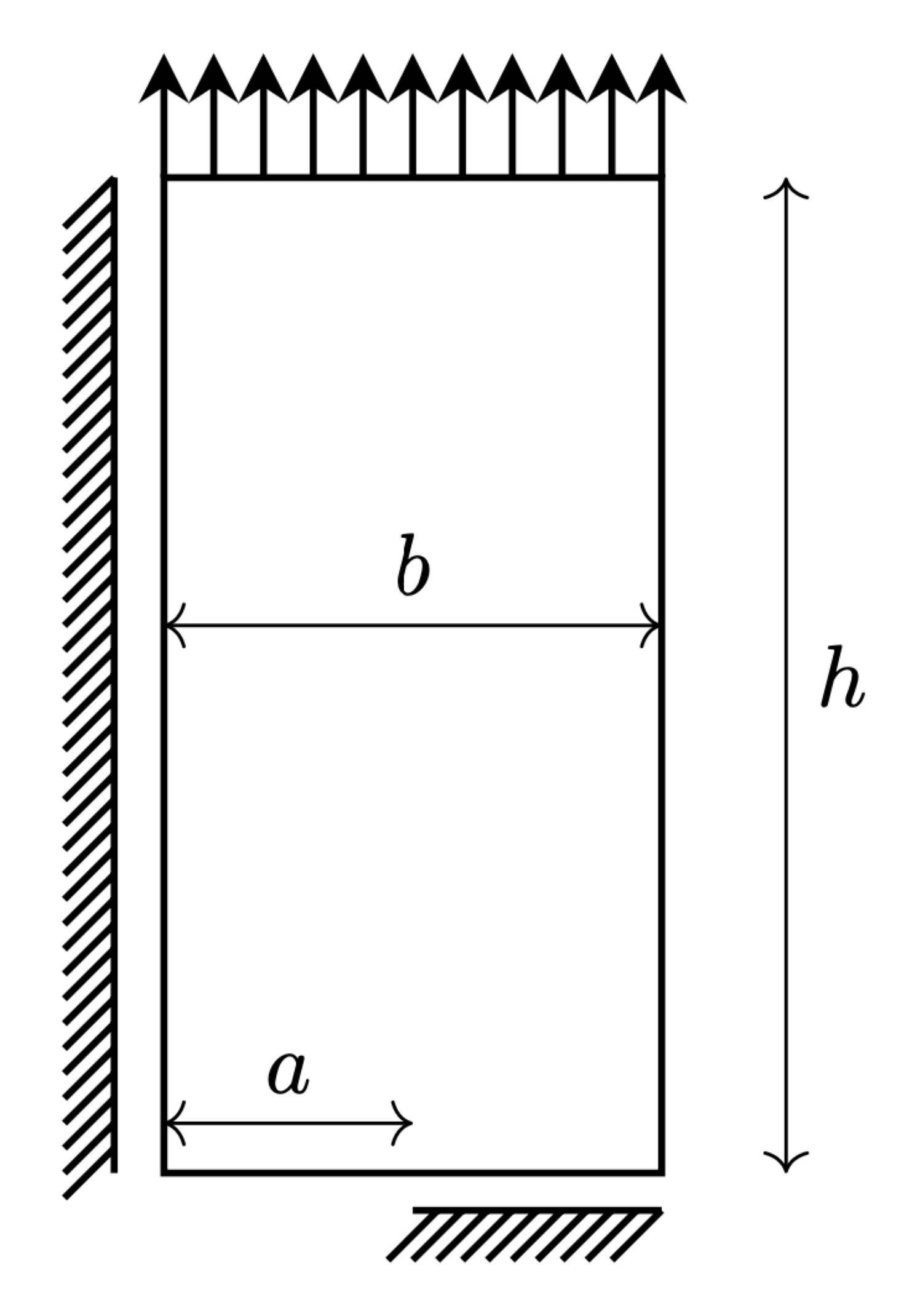
Purely elastic Finite Element model under displacement loading. To improve computational efficiency, a quarter-symmetry model is employed. The crack is explicitly defined in the mesh by adjusting the boundary conditions. A series of simulations are run, each with a different pre-defined crack length.

#           u/\/\/\/\/\/\       u/\/\/\/\/\/\
#            ||||||||||||        ||||||||||||
#            *----------*    o|\ *----------*
#            |          |    o|/ |          |
#            | 2a=a0    |    o|\ | a=a0     |
#            |   ----   |    o|/ *----------*
#            |          |             /_\/_\
#            |          |            oo oo oo
#            *----------*
#            /_\/_\/_\/_\
#     |Y    /////////////
#     |
#     *---X

The Young’s modulus, Poisson’s ratio, and the critical energy release rate are given in the table Properties. Young’s modulus \(E\) and Poisson’s ratio \(\nu\) can be represented with the Lamé parameters as: \(\lambda=\frac{E\nu}{(1+\nu)(1-2\nu)}\); \(\mu=\frac{E}{2(1+\nu)}\).

Material Properties

The material properties are summarized in the table below:

	VALUE	UNITS
E	210	kN/mm2
nu	0.3	[-]

Import necessary libraries

import numpy as np
import pyvista as pv
import pandas as pd
import matplotlib.pyplot as plt
import matplotlib.image as mpimg
import sys
import os
sys.path.insert(0, os.path.abspath('../../'))
plt.style.use('../../graph.mplstyle')
import plot_config as pcfg

import dolfinx
import mpi4py
import petsc4py
import os


img = mpimg.imread('images/symmetry_central_cracked.png')  # or .jpg, .tif, etc.
plt.imshow(img)
plt.axis('off')

(-0.5, 699.5, 1031.5, -0.5)

Import from phasefieldx package

from phasefieldx.Element.Elasticity.Input import Input
from phasefieldx.Element.Elasticity.solver.solver import solve
from phasefieldx.Boundary.boundary_conditions import bc_x, bc_y, get_ds_bound_from_marker
from phasefieldx.PostProcessing.ReferenceResult import AllResults

results_folder = "results_center_cracked_displacement_control"
if not os.path.exists(results_folder):
    os.makedirs(results_folder)

def run_simulations(i, a0):
    Data = Input(E=210.0,
                 nu=0.3,
                 save_solution_xdmf=False,
                 save_solution_vtu=True,
                 results_folder_name=os.path.join(results_folder,str(i)))

    divx, divy = 200, 600
    lx, ly = 1.0, 3.0
    msh = dolfinx.mesh.create_rectangle(mpi4py.MPI.COMM_WORLD,
                                        [np.array([0, 0]),
                                        np.array([lx, ly])],
                                        [divx, divy],
                                        cell_type=dolfinx.mesh.CellType.quadrilateral)

    def bottom(x):
        return np.logical_and(np.isclose(x[1], 0), np.greater_equal(x[0], a0))

    def top(x):
        return np.isclose(x[1], ly)

    def left(x):
        return np.isclose(x[0], 0)

    fdim = msh.topology.dim - 1 # Dimension of the mesh facets

    bottom_facet_marker = dolfinx.mesh.locate_entities_boundary(msh, fdim, bottom)
    top_facet_marker = dolfinx.mesh.locate_entities_boundary(msh, fdim, top)
    left_facet_marker = dolfinx.mesh.locate_entities_boundary(msh, fdim, left)

    ds_top = get_ds_bound_from_marker(top_facet_marker, msh, fdim)
    ds_bottom = get_ds_bound_from_marker(bottom_facet_marker, msh, fdim)
    ds_left = get_ds_bound_from_marker(left_facet_marker, msh, fdim)

    ds_list = np.array([
                    [ds_top, "top"],
                    [ds_bottom, "bottom"],
                    [ds_left, "left"],
                    ])

    V_u = dolfinx.fem.functionspace(msh, ("Lagrange", 1, (msh.geometry.dim, )))

    bc_top = bc_y(top_facet_marker, V_u, fdim, value=0.0)
    bc_bottom = bc_y(bottom_facet_marker, V_u, fdim, value=0.0)
    bc_left = bc_x(left_facet_marker, V_u, fdim, value=0.0)

    bcs_list_u = [bc_top, bc_bottom, bc_left]
    bcs_list_u_names = ["top", "bottom", "left"]

    def update_boundary_conditions(bcs, time):
        val = 1
        bcs[0].g.value[...] = petsc4py.PETSc.ScalarType(val)
        return 0, val, 0

    T_list_u = None
    update_loading = None
    f = None

    final_time = 1.0
    dt = 1.0

    solve(Data,
        msh,
        final_time,
        V_u,
        bcs_list_u,
        update_boundary_conditions,
        f,
        T_list_u,
        update_loading,
        ds_list,
        dt,
        path=None,
        quadrature_degree=2,
        bcs_list_u_names=bcs_list_u_names)


da=0.01
a = np.arange(0.0, 0.95+da, da)

run_simulation_bool = False

if run_simulation_bool:
    for i in range(0,len(a)):
        run_simulations(i, a[i])


    ###############################################################################
    # Load results
    # ------------
    compliance = np.zeros(len(a))
    E = np.zeros(len(a))
    for i in range(0,len(a)):
        print(f"Loading results for simulation {i} with crack length {a[i]} mm")
        simulation_folder = os.path.join(results_folder,str(i))
        S = AllResults(simulation_folder)
        compliance[i] = 2*S.energy_files["total.energy"]["E"][0]/S.reaction_files["bottom.reaction"]["Ry"]**2

    # %%
    # For this symmetric model, the compliance calculated here for the full specimen
    # is equivalent to that of a quarter-symmetry model, due to boundary conditions and loading.
    # Note: The variable 'a_saved' stores the half-crack length 'a' (not the total crack length 2a),
    # which is consistent with the convention used in the documentation and manuals.
    a_saved = a
    stiffness_complete_model = abs(1/compliance)

    # %%
    # Save processed results to file
    header = ["crack_length", "stiffness"]
    data_save = np.column_stack((a_saved, stiffness_complete_model))
    save_path = os.path.join(results_folder, "results.elasticity")
    np.savetxt(save_path, data_save, fmt="%.6e", delimiter="\t", header="\t".join(header), comments="")

else:
    # Load processed results from file
    save_path = os.path.join(results_folder, "results.elasticity")
    data_loaded = pd.read_csv(save_path, delim_whitespace=True, comment="#")
    a_saved = data_loaded["crack_length"].to_numpy()
    stiffness_complete_model = data_loaded["stiffness"].to_numpy()

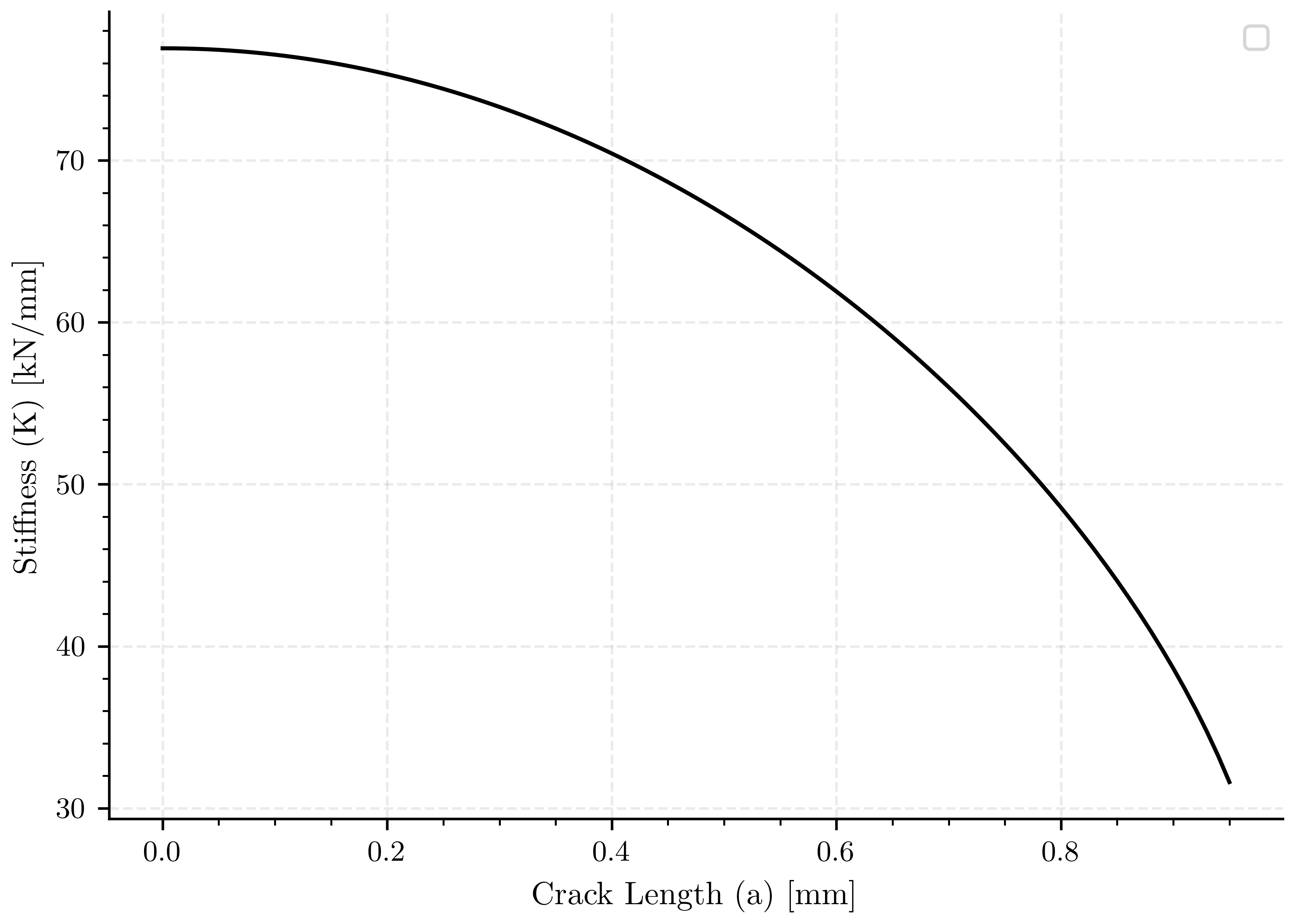
Crack length vs stiffness

fig, ax0 = plt.subplots()

ax0.plot(a_saved, stiffness_complete_model, 'k-')

ax0.set_xlabel(pcfg.crack_length_label)
ax0.set_ylabel(pcfg.stiffness_label)
ax0.legend()
plt.show()

/home/docs/checkouts/readthedocs.org/user_builds/phasefieldfatigue/checkouts/stable/examples/Elasticity/plot_center_cracked_displacement_control.py:211: UserWarning: No artists with labels found to put in legend.  Note that artists whose label start with an underscore are ignored when legend() is called with no argument.
  ax0.legend()

Visualization of Results

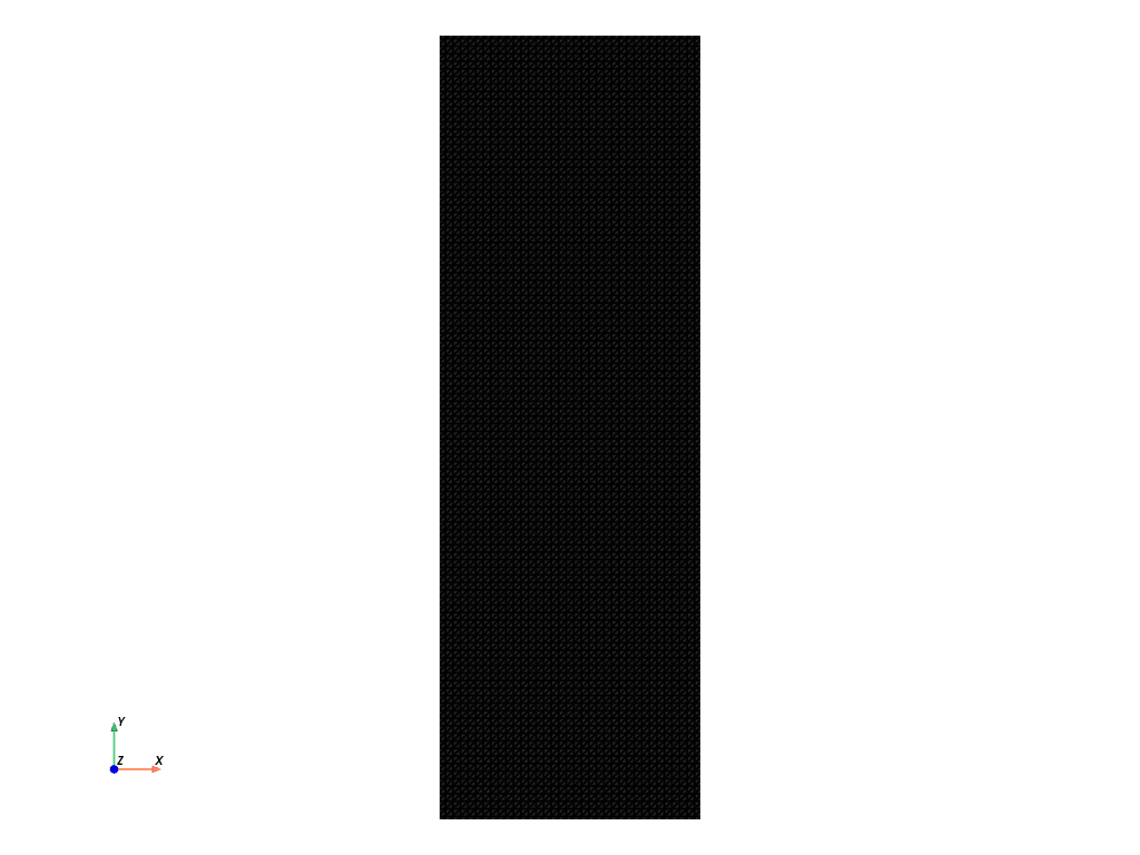
The following section visualizes the mesh and displacement field for two different simulations (indices 20 and 50). The mesh is shown first, followed by the displacement field, which is warped by the displacement vector for better visualization.

pv.start_xvfb()
file_vtu_1 = pv.read(os.path.join(results_folder, "20", "paraview-solutions_vtu", "phasefieldx_p0_000000.vtu"))
file_vtu_2 = pv.read(os.path.join(results_folder, "80", "paraview-solutions_vtu", "phasefieldx_p0_000000.vtu"))

Plot: Mesh

Display the mesh for the first simulation (index 20).

file_vtu_1.plot(cpos='xy', color='white', show_edges=True)

Static Scene

Interactive Scene

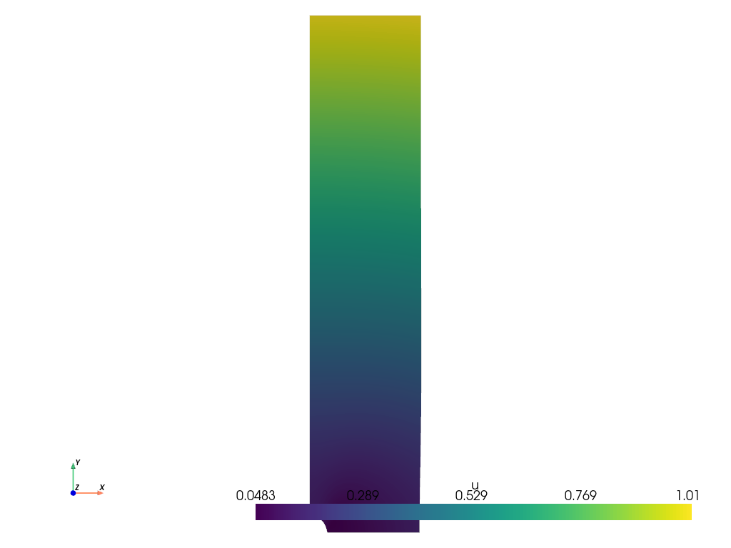
Plot: Displacement (Simulation 20)

Warp the mesh by the displacement vector for the first simulation and plot the displacement field.

warped_1 = file_vtu_1.warp_by_vector('u', factor=1.0)
warped_1.plot(scalars='u', cpos='xy', show_scalar_bar=True, show_edges=False)

Static Scene

Interactive Scene

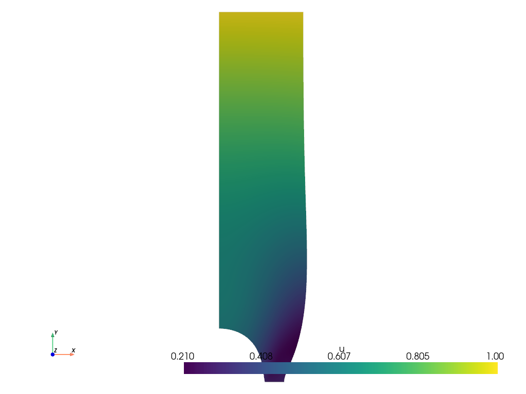
Plot: Displacement (Simulation 50)

Warp the mesh by the displacement vector for the second simulation and plot the displacement field.

warped_2 = file_vtu_2.warp_by_vector('u', factor=1.0)
warped_2.plot(scalars='u', cpos='xy', show_scalar_bar=True, show_edges=False)

Static Scene

Interactive Scene